

FSR 2026 H2
In a nutshell
Increased risk of serious events that could weaken financial stability
The Norwegian financial system is resilient. At the same time, the risk of serious events has increased. Geopolitical tensions and cyberattacks, high and rising government debt in many countries and uncertainty related to the consequences of artificial intelligence could cause economic and financial market stress. International stress could quickly affect Norway.
Most households have the financial capacity to cope with new economic shocks
Norwegian households are highly indebted, but debt growth has been slower than income growth in recent years. Debt-to-income (DTI) ratios have declined the most for households with the highest levels of debt. Over the past two years, wages have risen more than prices. For many households, this has strengthened purchasing power, improved debt-servicing capacity and also increased saving.
Higher interest rates are putting pressure on property values
Banks have substantial commercial real estate (CRE) exposures. Overall, CRE firms have strengthened their solvency in recent years, partly through property sales, equity injections and debt reduction. Higher interest rates are nevertheless putting pressure on property values ahead. Conditions remain challenging for real estate developers, with weak demand and high costs making few new construction projects profitable. Bankruptcies have increased, and banks report an increased risk of default in this sector.
Capital requirements are bolstering resilience
Norwegian banks are solid, have ample liquidity and low losses. Households and firms have ample access to credit. Capital buffer requirements, such as the countercyclical capital buffer, bolster the resilience of the Norwegian financial system.
The Committee’s assessment
Norges Bank’s Monetary Policy and Financial Stability Committee considers the Norwegian financial system to be resilient. Most households and firms have solid debt-servicing capacity, and debt-to-income (DTI) ratios have declined broadly across households. Overall, Norwegian firms are financially sound, but higher interest rates are putting pressure on property prices. At the same time, partly owing to geopolitical tensions, cyber threats, high and rising government debt in many countries and potential AI implications, the risk of serious events that could weaken financial stability has increased. Norwegian banks’ capital buffer requirements are bolstering the resilience of the Norwegian financial system to economic downturns.
Increased risk of serious events that could weaken financial stability
The international balance of risks is marked by geopolitical tensions. The conflicts in the Middle East and the closure of the Strait of Hormuz have pushed up energy and commodity prices. In spite of conflicts and considerable trade policy uncertainty, global economic activity has remained elevated, although economic growth has been slightly slower so far in 2026 than in 2025. A number of central banks have raised policy rates. Long-term interest rates have risen and are at multi-decade highs in a number of markets.
The policy rate in Norway has also been raised in 2026. Inflation has been above target for a number of years, and the rapid rise in business costs in recent years will likely contribute to keeping inflation elevated ahead. Higher prices for energy and various other commodities owing to the conflict in the Middle East are pushing up inflation both abroad and in Norway. In recent years, the policy rate has dampened economic activity, and capacity utilisation appears to be slightly below a normal level. However, most households are able to service debt by an ample margin, partly reflecting high employment. There is substantial uncertainty regarding the global economic outlook. Weaker global growth than assumed may lower demand for Norwegian exports and reduce investment in Norway.
The Committee considers the Norwegian financial system to be resilient. At the same time, the risk of serious events that could weaken financial stability has increased. In a turbulent world, the risk of targeted cyberattacks and other operational disruptions increases. Recently, more such incidents have occurred internationally. In a global, interconnected financial system, new external shocks can quickly affect the Norwegian financial system. An AI-driven market correction or a marked rise in long-term interest rates will result in lower asset values, and may result in higher risk premiums and higher funding costs for Norwegian banks. This may also reduce access to credit for households and firms.
Higher debt makes technology companies more vulnerable
High AI-related investment has contributed to underpinning global economic growth and has been a key driver of developments in both equity and fixed-income markets in 2026. High earnings and expectations of further growth have pushed up the equity prices of large technology companies in 2026 H1. Major equity indices have fallen in recent weeks, reflecting higher uncertainty about the framework conditions for data centre build-outs in the US and about whether the large AI investments will yield sufficient returns.
If expected AI-related productivity gains are realised, the technology could push up global growth markedly. At the same time, there is considerable uncertainty regarding the magnitude of these gains, how quickly they will materialise and how they will be distributed between countries, companies and others. AI-related investment is increasingly being financed by debt, particularly through bond markets, but also through banks and private credit funds. Increased debt financing makes markets more vulnerable if companies fail to meet the high expectations. This could trigger sharp falls in equity and bond prices and contribute to financial system turbulence.
High and rising government debt may cause market stress
Government debt is high and rising in many countries. Higher interest rates and steadily rising expenditure on eg defence and an aging population, combined with growing political divisions in many countries, make it difficult for governments to sufficiently tighten public budgets. An increase in uncertainty about government debt sustainability could lead to asset devaluations and higher risk premiums in global financial markets.
Highly leveraged investors can amplify and spread market stress
In recent years, price-sensitive investors such as hedge funds have become increasingly important in international financial markets, particularly in equity and government bond markets. These funds are often highly leveraged and may face liquidity difficulties during periods of severe market volatility, forcing them to fire-sell securities. Such sales can amplify market movements and impair market liquidity, and thereby also contribute to higher risk premiums elsewhere in the financial system.
Frontier AI models increase cyber risk
Operational resilience is essential for financial stability. In October, the Norwegian National Security Authority raised the cyber risk level to high, partly as a result of technological advances and a demanding threat landscape. AI can enhance the ability to manage cyber threats but can also enable faster and more sophisticated cyberattacks. In July, the European Systemic Risk Board (ESRB) warned that frontier AI models have increased systemic cyber risk. Norges Bank and Finanstilsynet (Financial Supervisory Authority of Norway) endorsed the warning. Increased digitalisation and increasing interconnectedness have made the financial system more dependent on shared technology and service providers. A serious operational failure or an extensive cyberattack could therefore affect many market participants simultaneously. Financial sector entities are making a considerable effort to strengthen the resilience of proprietary systems, and it is important that this work continues.
Most households have leeway to withstand new economic shocks
The high indebtedness of many households is a key financial system vulnerability. For a long period, debt rose faster than household income. Nevertheless, banks have incurred low losses on loans to households since the banking crisis in the 1990s, partly reflecting increased debt-servicing capacity from stronger purchasing power over time. At the same time, high debt, especially when combined with limited liquid assets, can increase the risk of sharp consumption cutbacks if interest rates rise, income is reduced or house prices fall markedly. This could weaken firms’ earnings and debt-servicing capacity. In recent years, debt has risen less than income. Analyses in this Report show that debt burdens have declined broadly across households and most for those with the highest debt-to-income (DTI) ratios.
Higher interest rates and high inflation tightened household finances in the years following the pandemic. However, most households have been able to service debt and cover necessary expenses out of current income by an ample margin. Over the past two years, wage growth has outpaced inflation. Many households’ purchasing power and debt-servicing capacity have improved, even when taking higher interest rates into account.
Many households have financial buffers that make them better able to cope with higher expenses or income loss. After declining in the years following the pandemic, there are signs that overall liquid buffers are increasing again. Over the past few years, households have increased their savings in bank deposits, funds and equities. This diversifies the financial buffers, but also makes them more vulnerable to financial market developments. In Norges Bank’s overall assessment, household vulnerabilities related to high debt have diminished somewhat.
Higher interest rates put pressure on property values
Norwegian firms’ financial positions were stable through 2025. Overall, Norwegian firms are financially sound. Profitability strengthened somewhat in 2025 after having weakened in pace with the rise in interest rates in recent years. Bankruptcy rates in most sectors are at approximately the same level as the average for the past decade.
A key financial system vulnerability is the high CRE exposure of Norwegian banks. In recent years, the rise in financing costs and the fall in property values have put pressure on both CRE firms’ profitability and solvency. However, CRE firms have strengthened their overall solvency over the past two years. A number of firms have adapted to a higher interest rate level by selling properties, injecting new equity and deleveraging. Analyses in this Report show that the share of particularly vulnerable firms with low solvency ratios and weak debt-servicing capacity fell last year.
Over the past year, yields in the office segment have remained fairly stable despite the rise in long-term interest rates. Strong demand from equity-financed investors and lower lending margins on CRE loans have likely contributed to keeping yields down. Market participants now report that demand from equity-financed investors is increasingly shifting towards other real estate segments, while lending margins have stabilised. Higher long-term interest rates are therefore expected to put pressure on property values ahead. Rising office vacancy rates are curbing the rise in rents, but few new office projects are expected to reach completion in the coming years, which will help sustain rents, particularly in central Oslo.
High construction and financing costs have dampened demand for new residential and commercial property in recent years and made conditions challenging for real estate developers. Bankruptcies have risen markedly, and a number of them have been among real estate developers with high bank debt. Weak demand and high costs mean that few new construction projects are profitable. Lower land values could help make projects financially viable. However, Norges Bank’s analyses show that land-related values remain elevated. There is considerable uncertainty surrounding developments in construction activity ahead. A number of Norges Bank’s Regional Network contacts point out that residential construction has troughed, but many report that the recovery keeps getting delayed.
Norwegian banks are solid
Banks are the most important source of financing for most households and firms in Norway, and bank deposits are important for both payments and saving. Norwegian banks are solid and satisfy capital and liquidity requirements by an ample margin.
Strong profitability is banks’ first line of defence against losses. Profitability has declined somewhat in 2026 but remains higher than the average for the past ten years. The decline mainly reflects lower net interest income. In Norges Bank’s lending survey for 2026 Q3, half of banks report an increased risk of breach of the terms of loan covenants and default on loans to real estate developers. Somewhat higher bank losses on construction exposures are expected in the year ahead. Overall, banks’ credit losses remain low, and they are also expected to continue to record low losses and strong profitability ahead.
Norwegian banks have ample access to both deposit and wholesale funding. Banks raise a substantial share of their funding in international markets, some of which is converted to finance lending in NOK. Severe market stress can lead to higher funding costs and liquidity difficulties for banks. Liquidity needs would primarily be in NOK, and banks are well equipped to manage liquidity stress in foreign currencies (see Financial Stability Report 2026 H1).
Cross-border interconnectedness between banks and non-bank financial institutions is increasing. Foreign hedge funds have become an important investor group in the Norwegian covered bond market. Fire sales by hedge funds as a result of market stress could lead to funding problems for banks and other participants that obtain funding in the Norwegian market.
Should global turbulence lead to a marked economic downturn in Norway, weaker corporate earnings and higher unemployment could weaken corporate and household debt-servicing capacity. In such a situation, both higher default rates and a marked decline in property prices that reduces the value of banks’ collateral can be expected. Credit losses could then become substantially higher than currently anticipated. Sound profitability and solvency provide banks with a solid basis for weathering higher losses.
Rapid advances in AI may increase cyber risk and place high demands on firms’ digital resilience. Norwegian financial institutions must have up-to-date systems and sufficient capacity to handle vulnerabilities and to adequately manage and control both their proprietary solutions and the parts of their IT operations that have been fully or partly outsourced to third parties. Norges Bank and Finanstilsynet monitor cyber risk developments and continuously assess the consequences for financial stability.
Capital requirements contribute to resilience
The European Commission is considering amendments to simplify European banking regulations and to better facilitate how banks meet financing needs in the real economy. Draft legislation is expected in 2027 H1 and will likely have implications for banks’ capital requirements and resilience. In the Committee’s view, there are good reasons to simplify the regulatory framework, but international regulatory standards must be safeguarded while national authorities retain a certain flexibility to address national vulnerabilities.
Norwegian banks’ capital buffer requirements should reflect the vulnerabilities in the Norwegian financial system and bolster resilience. In the event of a sharp economic downturn, buffer requirements can be reduced to mitigate the risk of tighter bank lending. The solvency stress test in Financial Stability Report 2026 H1 illustrates that banks can absorb large credit losses while maintaining lending.
Norges Bank sets the countercyclical capital buffer (CCyB) rate each quarter. At its meeting on 4 November 2025, the Monetary Policy and Financial Stability Committee decided to keep the CCyB rate unchanged at 2.5%.
Norges Bank also provides advice on the systemic risk buffer (SyRB) rate every other year. In May 2026, the Monetary Policy and Financial Stability Committee decided to advise the Ministry of Finance to maintain the SyRB rate at 4.5%, and in October, the Ministry decided to keep the rate unchanged at 4.5%.
Ida Wolden Bache
Pål Longva
Øystein Børsum
Steinar Holden
Hilde Christiane Bjørnland
1.1 Increased risk of serious events that could weaken financial stability
Geopolitical tensions and artificial intelligence influence the global economy
The international balance of risks is marked by geopolitical tensions. The conflicts in the Middle East and the closure of the Strait of Hormuz have pushed up energy and commodity prices. Despite conflicts and considerable trade policy uncertainty, global economic activity has remained buoyant, although economic growth so far in 2026 has been slightly lower than in 2025. A number of central banks have raised their policy rates, and market participants now expect interest rates to remain higher than previously assumed. Long-term interest rates have risen and are at multi-decade highs in a number of markets.
Substantial investment related to artificial intelligence (AI) has underpinned global economic growth, and the technology may yield productivity gains. At the same time, increased use of AI will likely lead to change in demand for different types of labour, and there is considerable uncertainty about the extent and pace of this restructuring.
Increased risk of serious events that could weaken financial stability
Although financial markets have so far proven robust, and banks are generally well capitalised, the IMF’s October Global Financial Stability Report points out that lower fiscal headroom and increased interconnectedness between banks and highly leveraged NBFIs1 may amplify the effect of shocks. As potential triggering shocks, the IMF points in particular to an AI-driven market correction, a further marked rise in long-term interest rates and severe cyberattacks that affect critical functions or result in a serious loss of confidence. The European Systemic Risk Board (ESRB) also assesses that risks to financial stability have increased.2
Global economic developments affect financial stability in Norway
The policy rate in Norway has also been raised. Inflation has been above target for a number of years, and the rapid rise in business costs in recent years will likely contribute to keeping inflation elevated ahead. Higher prices for energy and various other commodities owing to the conflicts in the Middle East are also pushing up inflation. In recent years, the policy rate has dampened economic activity, and capacity utilisation appears to be slightly below a normal level (see Monetary Policy Report 3/2026). The krone has appreciated against many currencies in 2026, and the Oslo Børs benchmark index has risen.
New international shocks can affect the Norwegian financial system both through the real economy and financial markets (Chart 1.1). Should geopolitical tensions intensify or the economic gains from AI prove smaller than expected, international growth prospects may weaken. Weaker global growth may result in lower demand for Norwegian exports and reduced investment in Norway, which in turn may weaken earnings and debt-servicing capacity among Norwegian firms. An AI-driven market correction or a marked rise in long-term interest rates will result in lower asset values and may result in higher risk premiums and higher financing costs for Norwegian banks and firms that obtain financing abroad. This may also reduce access to credit for households and firms. Adaptation among highly leveraged NBFIs may amplify and propagate stress across markets. Strong resilience in the Norwegian financial system dampens the risk of vulnerabilities amplifying economic downturns (see “Key vulnerabilities in the Norwegian financial system”).

Norges Bank’s systemic risk survey conducted in October shows that Norwegian financial market participants consider geopolitical risk and cyberattacks to be the main sources of risk to the Norwegian financial system (Chart 1.2). These have been the two most important sources of risk highlighted by the survey’s respondents over the past two years. Overall, the respondents assess that the likelihood of an incident with a substantial impact on the financial system occurring in the next three years has increased somewhat. However, they are highly confident that the Norwegian financial system will remain stable.
Norges Bank’s October 2026 systemic risk survey. Which source of risk do you consider most likely?4
Frontier AI models increase cyber risk
Operational resilience is essential for financial stability. Norway’s financial infrastructure is secure and efficient, but Norway’s financial system is also vulnerable to cyberattacks. Increased digitalisation and increasing interconnectedness have made the financial system more dependent on shared technology and service providers. A serious operational failure or an extensive cyberattack could therefore affect many market participants simultaneously and disrupt critical financial services.
In October, the Norwegian National Security Authority raised the cyber risk level to high, partly as a result of technological advances and a demanding threat landscape. Frontier AI models enable threat actors to find vulnerabilities and conduct cyberattacks more rapidly and on a greater scale than before. In July, the ESRB therefore published a warning about higher systemic cyber risk.5 The ESRB pointed out that over time, frontier AI models are likely to eventually also strengthen cyber resilience, but that in the short to medium term the technology provides a relative advantage to threat actors.
More autonomous AI agents may also give rise to new forms of cyber risk. Such agents can perform complex tasks with limited human involvement and act in unforeseen or undesirable ways. Events over the past year have shown that AI agents can autonomously attempt to circumvent security mechanisms and gain access to restricted systems. AI can therefore increase cyber risk both through threat actors’ use of the technology and through autonomous action by AI agents.
This cyber threat landscape is also relevant for the Norwegian financial system. Norges Bank and Finanstilsynet (Financial Supervisory Authority of Norway) endorsed the warning published by the ESRB.6 Rapid technological advances require firms to maintain a high level of digital resilience. Norwegian financial institutions must have up-to-date systems and sufficient capacity to address vulnerabilities and adequately manage and control both proprietary solutions and those parts of their IT operations that have been fully or partly outsourced to third parties. Norges Bank monitors cyber risk developments as part of its work on financial stability and supervises security and contingency preparedness in key payment and settlement systems. The Bank also conducts exercises and analyses to assess how serious cyber incidents can affect critical financial services and propagate through the financial system. Together with Finanstilsynet, Norges Bank follows up the digital resilience of financial institutions through eg testing and dialogue. See further discussion in the Financial Infrastructure Report 2026.
Higher debt makes technology companies more vulnerable
International financial markets are increasingly influenced by developments in the AI sector. Expectations of continued strong growth in demand for AI services have accelerated the build-out of data centres and other AI-related infrastructure. Over the past year, high earnings and expectations that AI investment will contribute to further earnings growth have lifted equity prices in the large technology companies. These developments have lifted the US equity market in particular, where technology companies account for a large share of the market value of major equity indices (Chart 1.3). Recently, developments have been more volatile. Increased uncertainty about the profitability of extensive AI investment has contributed to falling equity prices in markets with a high proportion of technology companies, including in the US and Japan (Chart 1.3).
Equity indices. January 2025 = 1007
The large technology companies that account for much of the build-out of AI-related infrastructure, ie hyperscalers, have historically had low debt. However, the scope of AI investment plans has increased the need for debt financing, primarily from the bond market, but also from private credit funds and banks.8 According to the IMF, hyperscalers’ share of global investment-grade corporate bond issuance increased from less than 1% in 2024 to close to 10% in 2026.9
Uncertainty about the profitability of AI investment has increased recently. Debt risk premiums of some data centre and computer chip firms with low credit ratings have risen markedly. Higher debt makes technology companies more dependent on sufficient future earnings from AI investment. This may also increase systemic risk as many financial system participants, eg banks, hedge funds and other large corporate bond investors, such as insurance companies and pension funds, are exposed to AI sector developments. If profitability expectations for AI investment weaken considerably, this could lead to a concurrent marked repricing of both equity and credit markets.
Financial relationships have also become closer within the AI value chain.10 Some firms invest in or lend to other firms while also entering into agreements for the future purchase of the latters’ services. Such relationships can contribute to problems in one firm spreading to other parts of the value chain.
AI investment growth has also contributed to extensive data centre build-out in Norway. Many of the data centres are owned by foreign firms that largely obtain financing from international capital markets. So far, Norwegian banks therefore have limited direct exposure to these firms. At the same time, equity and credit market investors are exposed to these developments. Norwegian households have increased their investment in equities and mutual funds in recent years, and a marked fall in share prices could reduce their financial buffers (see Section 2.3). A market correction would also lead to valuation losses for Norwegian asset managers and funds with substantial investment in international equity markets. Norges Bank conducts stress tests of the investment portfolio of the Government Pension Fund Global (GPFG).11 In one of the 2025 scenarios, AI did not meet the market’s productivity gain expectations, resulting in lower expected cash flows and higher equity risk premiums. Under this scenario, the value of the GPFG fell by 35%.12
High and rising government debt may cause market stress
Long-term sovereign bond yields have risen since Financial Stability Report 2026 H1 (Chart 1.4). The rise reflects rate hikes by many central banks and persistently high market-implied policy rate expectations ahead. In addition, various measures of the term premium have increased. Large budget deficits and rising government debt in many countries, as well as a marked rise in hyper-scalers’ debt issuance, have led to an increased supply of long-term bonds. At the same time, demand from central banks and other traditional investors such as pension funds and insurance companies has declined. More price-sensitive investors such as hedge funds therefore account for a growing share of the investor base13 and may require higher compensation for holding long-term bonds. Long-term inflation expectations have also been fairly stable, meaning that the increase in nominal interest rates likely reflects an increase in real interest rates.
10-year government bond yields in selected countries. Percent14

Recently, the sustainability of public finances has received renewed focus in financial markets. In the US, large budget deficits and increasing interest expenses are expected to increase government debt considerably in the coming decade. In early October, ten-year US government bond yields rose to above 5.3%, the highest level since 2002. In Europe, the rise in yields has been most pronounced in France. Weaker growth prospects, higher spending on eg defence and higher interest expenses, as well as increasing political divisions in many countries, are making it difficult for governments to sufficiently tighten public budgets. The spread between French and German ten-year government bond yields has increased markedly.
Norwegian long-term yields are largely influenced by developments in international bond yields. Norwegian long-term yields have risen in 2026, but less than in many other European countries. The large movements in government bond yields have lifted fixed income market volatility indicators somewhat (Chart 1.5). Credit spreads have increased somewhat in the US and euro area, in particular for firms with low credit ratings, but also for banks’ wholesale funding. At the same time, European bank equity prices have fallen, reflecting the fact that government bonds are important references for the pricing of other financial instruments and their use as collateral for loans and derivatives. In many countries, banks also have large government bond holdings. Higher government bond yields reduce the value of banks’ holdings and can contribute to higher funding costs, as well as tighter credit standards for households and firms.

Turbulence in international government bond markets can also have implications for financial stability in Norway. During the European sovereign debt crisis in 2011 and 2012, Norwegian banks’ funding costs rose markedly. Higher risk premiums for banks’ wholesale funding can result in higher financing costs, as well as tighter credit standards for households and firms. The rise in long-term yields puts pressure on both debt-servicing capacity and asset values in commercial real estate (CRE), which can give rise to higher bank losses (see discussion in Section 3).
Highly leveraged investors can amplify and spread market stress
An AI-related market correction or a marked further rise in government bond yields can trigger considerable movements in financial markets. In recent years, price-sensitive market participants such as hedge funds have become increasingly important in international financial markets, particularly in the equity and government bond markets. Hedge funds are often highly leveraged and may, in the event of severe market volatility, experience liquidity problems and be forced to sell securities. Such divestment can amplify market movements and weaken market liquidity. At the same time, hedge funds finance a large share of their highly leveraged investments with bank debt. In periods of severe market turbulence, the close linkages to banks can propagate stress across different parts of the financial system.
Significant market movements internationally may also have consequences for the Norwegian financial system via NBFIs with exposures abroad. During the market turbulence in connection with the outbreak of the pandemic in 2020, falling international equity prices contributed to a substantial weakening of the krone. This weakening increased the collateral requirements on FX swaps that asset managers use to currency hedge foreign investment and resulted in a substantial liquidity need. Bond sales to cover this need pulled down market liquidity and pushed up risk premiums in the Norwegian bond market.16 Such adaptations can amplify market turbulence and weaken market liquidity, thereby posing a financial stability risk.
In recent years, foreign hedge funds have increased their ownership share in the Norwegian covered bond market (see Financial Stability Report 2026 H1). Covered bonds are an important source of wholesale funding for Norwegian banks. Should hedge funds be forced to fire-sell covered bonds, the result could be major price fluctuations and weakened liquidity in the covered bond market. This could in turn weaken funding conditions for Norwegian banks and other bond issuers.
The international private credit market has grown substantially and become an increasingly important source of corporate financing. In Norway, this market is still small, but activity levels have increased in recent years, particularly through lending from foreign funds.17 Although private credit operates outside the traditional banking system, banks may have indirect exposure through credit lines and other financing facilities to private credit funds. However, the exposure of the Norwegian banking sector to such structures appears to be very limited.
Stablecoin use is growing but does not pose a risk to financial stability in Norway
Stablecoins are cryptoassets designed to maintain a stable value against a reference asset. They are mostly used for cryptoasset investment, but their use is also growing in international payments and payments requiring programmability. Stablecoins may provide benefits within such areas, but they also lack some of the characteristics of general-purpose means of payment (see further discussion in Financial Infrastructure Report 2026).
In Norway, stablecoins are little used. Norges Bank’s cryptoasset surveys from 2024 and 2026 show limited awareness and use of stablecoins among the Norwegian public.18 Exposures among Norwegian financial institutions are also limited.
Stablecoin issuers hold reserves in the form of bank deposits and securities. Large redemptions can trigger fire sales of reserve assets and propagate stress to other parts of the financial system. The European Markets in Crypto-Assets Regulation (MiCAR) sets requirements for the reserve assets and helps mitigate risk. The Regulation has been transposed into Norwegian law from 1 July 2025 through the Cryptoassets Act. However, further regulatory development is needed. In 2026, the European Commission conducted a consultation on the review of MiCAR.19 The consultation response from the European System of Central Banks (ESCB) included a recommendation to remove the minimum percentages of the reserves that must be held as bank deposits. The ESCB pointed out that such reserve requirements create a direct link between stablecoin issuers and credit institutions20.
Cryptoasset theft may result in substantial losses and weaken confidence in the crypto market. In October 2026, around USD 6bn was stolen from Binance, the world’s largest crypto exchange, much of it in stablecoins. For the time being, major international crypto platforms, such as Binance, have limited connections to the Norwegian financial system. Closer interconnectedness between the crypto market and the traditional financial system could increase the risk that losses and loss of confidence will have implications for financial stability, also in Norway.
1 Non-bank financial institutions or intermediaries. The term includes not only traditional asset managers, such as insurance, pension funds and various other funds, but also hedge funds and other special purpose vehicles (SPVs).
2 See Outcomes of the 63rd General Board meeting of the European Systemic Risk Board – 1 October 2026.
3 The chart shows examples of how global economic developments can affect financial stability in Norway. It does not provide an exhaustive overview of the mechanisms.
4 Based on Norges Bank’s systemic risk survey from October. A selection of participants in the Norwegian financial system take part in the survey, and the responses reflect their risk assessments at the time the survey was completed.
The chart shows the most likely risk in the Norwegian financial system according to respondents.
5 See ESRB press release of 7 July 2026: Frontier AI models could strain cyber resilience in the financial system, ESRB warns.
6 See Norges Bank news item of 7 July 2026: The European Systemic Risk Board (ESRB) warns against frontier AI models.
7 Period: 1 January 2025–6 November 2026.
8 For more on the AI financing and linkages to private credit, see Aldasoro, I., S. Doerr and D. Rees (2026) "Financing the AI boom: from cash flows to debt". BIS Bulletin 120, 7 January 2026.
9 See International Monetary Fund (2026) “Resilience, Risk, and Transformation”. Chapter 1 and Background Analysis 1.1 in Global Financial Stability Report. IMF, October 2026.
10 For more on the financial relationships, see Frost, J.,R. Kansal et al. (2026) “Circular relationships among AI firms”. BIS Bulletin 137, 1 October 2026.
11 For more information about risk management in the GPFG, see Norges Bank Investment Management “Risk management”.
12 For more information about the scenarios and their results for the value of the GPFG, see Norges Bank Investment Management (2025) “Stress testing”.
13 According to the IMF, price-sensitive investors, ie investment funds, foreign investors and households, hold at least half of all US, Japanese, European and UK government debt. See the International Monetary Fund (2026) “Global Financial Markets Confront the War in the Middle East and Amplification Risks”. Chapter 1 of the Global Financial Stability Report. IMF, April 2026.
14 Period: 1 January 2000–6 November 2026.
15 Left panel panel:
Period: 1 January 2020–6 November 2026.
Right panel:
Period: 1 January 2022–6 November 2026.
16 See box “Asset managers faced liquidity stress during the foreign exchange market turbulence in March” in Financial Stability Report 2020, page 20.
17 For more information on private credit in Norway, see Iden, A.E., T.F. Tho and I.L. Tobiassen (2026) “Private credit in Norway”. Staff Memo 4/2026. Norges Bank.
18 See Norges Bank (2024) Survey on crypto-assets in Norway, Norges Bank Memo 2/2024 and Norges Bank (2026) Survey on crypto-assets in Norway, Norges Bank Memo 6/2026. The surveys covered individuals, not institutions and firms.
19 See consultation from the European Commission between 20 May and 30 September 2026. Targeted consultation on the review of MiCA Regulation – Finance
20 For more details on the recommendations, see the consultation response from the ESCB, September 2026: ESCB response to the European Commission’s targeted consultation on the Markets in Crypto-Assets Regulation (MiCAR)
1.2 Norwegian banks are resilient
Slightly weaker bank profitability
International shocks and market stress may have implications for the funding conditions and loss prospects of Norwegian banks. Banks’ funding markets have functioned well since the May Report. Turbulence in international fixed-income markets has contributed to a slight increase in risk premiums for banks’ wholesale funding in the past couple of months. At the same time, deposit-to-loan ratios are stable. Norwegian banks satisfy capital and liquidity requirements by an ample margin.
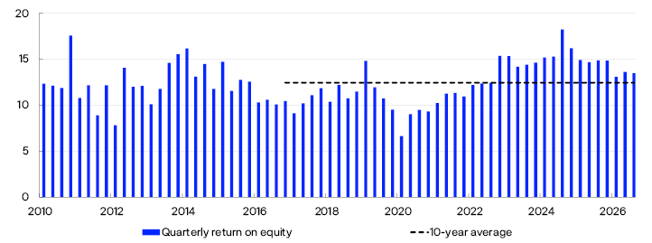
Profitable operations are banks’ first line of defence against losses. Norwegian banks’ return on equity has been high in recent years (Chart 1.6). Increased net interest income and low losses in particular have pushed up profitability. Higher net interest income reflects higher interest rates in the wake of the pandemic21 Profitability has declined slightly in 2026 but remains high.
Annualised quarterly return on equity. Percent22
Banks’ total credit losses have remained low and are in line with 2025 levels (Chart 1.7). Overall credit losses on corporate exposures are expected to increase slightly in 2026 and 2027 but to remain at low levels. Even though several key financial figures improved last year, the current situation is weighing on the liquidity of many real estate developers, and continued low construction activity is expected to result in higher losses on corporate exposures. Prospects for higher financing costs and lower rental income mean that losses on banks’ CRE exposures are also expected to increase slightly but to remain low.
Credit losses as a share of gross loans to customers. Percent23
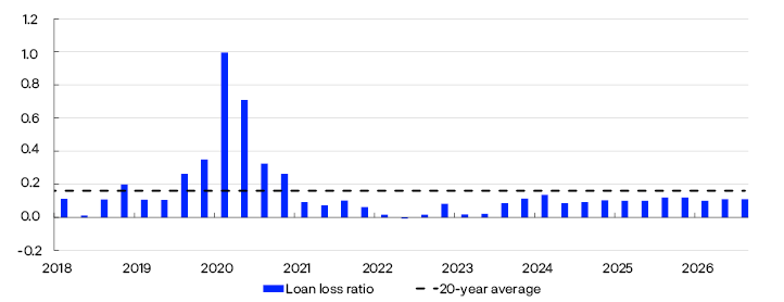
Losses on loans to households are low. Higher real income has strengthened household debt-servicing capacity in recent years, and the loss rate on household exposures is expected to remain at a low level.
Households and firms have ample access to credit
Norwegian banks’ financial strength gives them the flexibility to extend loans to creditworthy firms and households, even in the event of market stress and higher losses. In Norges Bank’s lending survey for 2026 Q3, banks reported unchanged credit standards, broadly unchanged household credit demand and slightly weaker corporate demand. In Q4, banks expect household credit demand to be broadly unchanged and corporate demand to decline slightly further. Bond market activity has been at a normal level this autumn. Credit spreads for investment-grade firms increased somewhat in October but are close to the average for the past decade. In Norges Bank’s assessment, households and firms have ample access to credit.
Capital requirements are bolstering resilience
The Common Equity Tier 1 (CET1) ratios of Norwegian banks are well above total capital requirements. Looking ahead, continued high profitability and low losses are expected to help keep banks’ capital adequacy ratios at a high level. The solvency stress test in Financial Stability Report 2026 H1 shows that banks can absorb large credit losses while maintaining lending to households and firms, and that they therefore will not amplify an economic downturn.
Capital buffers form part of banks’ overall capital requirements and are important macroprudential policy instruments. Norges Bank sets the countercyclical capital buffer (CCyB) rate each quarter and provides the Ministry of Finance with advice on the systemic risk buffer rate at least every other year.
The CCyB is intended to reflect the assessment of cyclical vulnerabilities in the financial system and mitigate the risk of banks amplifying an economic downturn. At its meeting on 4 November 2026, Norges Bank’s Monetary Policy and Financial Stability Committee decided to keep the countercyclical capital buffer rate unchanged at 2.5 percent.
The SyRB is intended to help ensure that banks hold sufficient capital to withstand downturns, and should reflect the structural vulnerabilities in the financial system, ie persistent features that change little from year to year. In May, Norges Bank advised the Ministry of Finance to maintain the SyRB rate at 4.5% for all exposures in Norway. In November, the Ministry of Finance decided to keep the requirement unchanged.24
The Ministry of Finance has stipulated a floor for average risk weights for residential and CRE mortgages in banks that use an internal ratings-based approach to calculate their capital requirements. Such floors serve as a backstop that prevent banks’ capital levels from becoming too low as a result of a fall in risk weights. Excessively high floors may, however, weaken both the risk sensitivity of the capital requirements and the incentives for sound risk management. In a consultation letter of 21 September 2026 from the Ministry of Finance, Finanstilsynet proposes maintaining the current risk weight floor levels.25 In its consultation response, Norges Bank has no reservations to the proposal.26
In Norway, the financial system has proven resilient to major market shocks and higher interest rates in recent years. The introduction of new regulation in Norway and abroad following the financial crisis has bolstered resilience both internationally and domestically. The European Commission is currently considering amendments to simplify European banking regulations and to better facilitate how banks meet financing needs in the real economy. This work includes the interaction between different capital requirements, macroprudential policy instruments and crisis management requirements. Draft legislation is expected in 2027 H1 and will likely have consequences for banks’ capital requirements and resilience. In Norges Bank’s view, there are good reasons for simplifying the regulatory framework, but international regulatory standards must be safeguarded while national authorities retain a certain flexibility to address national vulnerabilities.
21 Policy rate hikes increase banks’ interest income more than interest expenses because banks have more interest-bearing assets than interest-bearing liabilities (equity effect). In addition, banks often raise average lending rates more than average deposit rates (interest margin increase).
22 Period: 2010 Q1–2026 Q3.
Figures for the six largest Norwegian-owned banking groups.
For comparability, the sample has been adjusted retrospectively for major mergers/acquisitions; ie for periods prior to a merger/acquisition, figures for the merged banks have been included.
23 Period: 2018 Q1–2026 Q3.
All banks and mortgage companies in Norway. Annualised. Branches and subsidiaries abroad are not included.
24 See news item about the decision made by the Ministry of Finance on 2 November 2026: Kravet til systemrisikobuffer videreføres [SyRB requirement maintained] (in Norwegian only).
25 See news item of 21 September 2026 about the Ministry of Finance’s consultation: Høring – gulv for risikovekting av boliglån og næringseiendomslån [Consultation – risk weight floor levels for mortgages and CRE loans] (in Norwegian only).
26 See Norges Bank (2026). Høringsvar fra Norges Bank – gulv for risikovekting av boliglån og næringseiendomslån [Consultation response – risk weight floor levels for mortgages and CRE loans] (in Norwegian only). 11 November 2026.
Key vulnerabilities in the Norwegian financial system
The economy is regularly exposed to shocks that affect both the real economy and the financial system. Promoting financial stability means ensuring sufficient financial system resilience to absorb such shocks. In this work, Norges Bank focuses on assessing systemic risk. The financial system should contribute to stable economic developments by channelling funds and offering savings products, executing payments and distributing risk efficiently. Systemic risk is the risk of disruption to the financial system’s ability to perform these functions.
The level of systemic risk depends on a number of factors. The risk of economic shocks, such as geopolitical tensions, pushes up systemic risk. Financial system vulnerabilities further increase systemic risk. At the same time, the financial system can be designed to be more resilient to shocks. In response to financial system vulnerabilities, a number of measures have been introduced to strengthen resilience, including requirements for banks’ solvency, liquidity and credit standards.


Many Norwegian households are highly indebted. This vulnerability has built up over time as debt levels rose more than household income over an extended period. However, banks’ losses on household exposures have been low in the past three decades, reflecting the fact that increased purchasing power over time has improved debt-servicing capacity. At the same time, high debt, especially when combined with low liquidity, can increase the risk of sharp consumption cutbacks if interest rates rise, household income is reduced or house prices fall markedly. Should multiple such shocks coincide, consumption cutbacks could weaken firms’ earnings and debt-servicing capacity, leading to higher bank losses on corporate exposures and amplifying the downturn through tighter credit standards.
In recent years, debt growth has been slower than income growth. DTI ratios have declined broadly across households and most for those with the highest ratios. In Norges Bank’s overall assessment, Norwegian household vulnerabilities related to high debt is somewhat reduced (see Section 2 for a further discussion of household sector vulnerabilities).
Another key vulnerability is banks’ high share of CRE exposure. This share has remained stable in recent years. Experience from banking crises in Norway and abroad has shown that losses on CRE exposures have been an important factor behind solvency problems in the banking sector. Banks incurred losses on approximately one third of their CRE loans during the banking crisis in the period 1988–1993. In recent years, the rise in financing costs and the decline in property values have put pressure on CRE firms’ profitability and solvency. However, CRE defaults have remained stable at a low level, and over the past two years, CRE firms overall have strengthened their solvency. A number of firms have adapted to a higher interest rate level by selling properties, injecting new equity and paying off debts. Higher long-term interest rates and weaker demand for office space pull in the direction of weaker developments in profitability and property values ahead. A marked increase in long-term interest rates and risk premiums could weaken both debt servicing capacity and property values. If a price fall leads to lower pledged collateral values than the carrying amount of loans, banks may incur losses if the debt is defaulted on. See Section 3 for a more detailed discussion of the CRE sector.
Furthermore, banks in Norway are interconnected through interbank exposures and have common or similar securities in their liquidity reserves. Covered bonds account for a large part of banks’ liquidity reserves. If a number of banks need liquidity and have to sell such a large quantity of covered bonds that the value of the bonds falls, the value of covered bond holdings in the liquidity reserves of all other banks will also fall. Cross-holdings of bonds mean that banks fund other banks. If banks were to withdraw collectively as buyers of covered bonds during market stress, this could weaken their ability to obtain new covered bond funding and could more easily lead to liquidity problems spreading and becoming self-reinforcing (see Financial Stability Report 2026 H1).
Digitalisation makes the financial system more efficient but also leads to cyber vulnerability. Artificial intelligence (AI) increases cyber risk by strengthening attackers’ ability to swiftly and efficiently detect and exploit vulnerabilities before they are addressed. Concentration, complexity and interconnectedness may amplify the consequences of a cyberattack that then spreads rapidly and widely across the financial system. In a turbulent world, the risk of targeted cyberattacks and other operational disruptions increases. Cyberattacks that disrupt critical functions or lead to a broad loss of confidence may threaten financial stability. Adequate contingency arrangements are important for managing such serious situations (see Financial Infrastructure Report 2026).
Furthermore, banks’ substantial exposures to sectors that are particularly vulnerable to climate transition are a financial system vulnerability. The Norwegian business sector must adapt to climate change and the use of new forms of energy. There is considerable uncertainty about the cost of such a transition, and some firms may see their earnings weaken. If many firms are adversely affected, this may result in higher bank losses. More extreme weather events can also increase insurance premiums and other housing-related costs and thereby impact household resilience.
2.1 Debt-to-income ratios have declined and are levelling off
Many Norwegian households have high debt-to-income (DTI) ratios, and Norges Bank has long considered this to be a key vulnerability in the Norwegian financial system. Since the banking crisis in the 1990s, few households have defaulted on their debt, even in downturns. At the same time, high debt levels can increase the risk of sharp consumption cutbacks if interest rates rise, household income is reduced or house prices fall markedly. Analyses from Norges Bank indicate that households with high DTI ratios tighten consumption more than households with low DTI ratios, both when faced with higher interest rates and high inflation, and when house prices fall markedly.1 This channel is amplified if households have small liquid buffers or limited access to credit. Such cutbacks can affect firms’ earnings and in turn lead to higher corporate credit losses among banks. Both DTI ratios and the size of liquid buffers therefore have implications for household vulnerability.
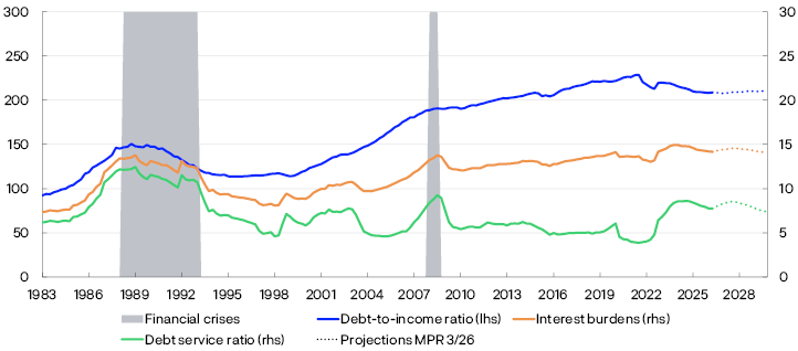
Norwegian household DTI ratios2 rose over many years and are high both historically and compared with other countries (Chart 2.1). Over the past five years, debt growth has been slower than income growth, and the overall household DTI ratio has declined. The debt service ratio and the interest burden have also declined slightly over the past two years, after rising substantially in pace with higher interest rates in the preceding years. Looking ahead, household debt is expected to rise broadly in pace with income, and that the DTI ratio therefore will change little. Household interest burdens are expected to increase somewhat in the near future as a result of higher interest rates, before gradually falling back.
Percent3
According to Finanstilsynet’s (Financial Supervisory Authority of Norway) Residential Mortgage Survey for 2025, the average DTI ratio increased for new mortgages and for the share of new mortgages issued with loan-to-value (LTV) ratios close to 90%. This reflects the increase in the Lending Regulations’ maximum LTV ratio requirement from 85% to 90%. This year’s survey shows that both the average DTI ratio and the share of new loans with LTV ratios close to 90% have increased somewhat further.4
Banks can use flexibility quotas to grant loans that deviate from one or more requirements in the Lending Regulations.5 After the regulatory amendment in 2025, banks’ use of flexibility quotas related to the LTV ratio requirement declined (Chart 2.2). In Oslo, the decline was less pronounced than in the rest of Norway, reflecting the fact that the DTI ratio is the main binding requirement for borrowers in Oslo. At the same time, use of flexibility quotas related to the DTI requirement has increased.
Share of new mortgages that deviate from each requirement in the Lending Regulations. Perc4ent6

Increased household purchasing power
Following the decline in 2022 and 2023, average household real disposable income increased again in 2024 and 2025 (Chart 2.3, left panel). Growth in real disposable income continued through 2026 H1, partly driven by the rise in wage income, pensions and government benefits. Growth ahead is expected to be lower than in the past two years but at broadly the same level as the average for the past 10 years (see Monetary Policy Report 3/2026).

Household credit growth picked up again in 2024 and 2025 after a period of slowing growth (Chart 2.3, right panel). So far in 2026, credit growth has levelled off, with a 12-month rise of 4.5% in September. The higher interest rate level and expectations of higher mortgage rates ahead may have curbed credit demand.8 Despite the rise in 2024 and 2025, credit growth remains lower than before the pandemic. In Norges Bank’s lending survey, banks report broadly unchanged residential mortgage demand in 2026 Q3, and they expect no change in Q4.9
Consumer debt10 only accounts for slightly less than 4% of overall household debt, but has historically accounted for the largest share of banks’ credit losses on household exposures.11 Growth in household consumer debt was particularly strong in 2022 and 2023, but has slowed in recent years. Consumer credit growth has been driven by an increase in instalment loans. Despite increased credit card use, interest bearing credit card debt has trended downwards since 2022.
The decline in household debt burdens is broad-based
Vulnerabilities related to high household debt depend not only on the overall debt burden but also on how debt is distributed across households. Microdata are therefore used to examine more closely how DTI ratios have developed across household groups.
Norwegian households have historically accumulated substantial debt, particularly related to home purchases in the household formation phase. DTI ratios therefore vary between households in different age groups (Chart 2.4, left panel). In recent years, DTI ratios have declined in all age groups. Since 2021, the decline has been most pronounced among households under the age of 35, which also have the highest DTI ratios.
Debt as a share of after-tax income by age group. Percent12

At the same time, there are wide differences in DTI ratios within each age group (Chart 2.4, right panel). In the 25–34 age group, 10% of households had DTI ratios higher than 5.6 times after-tax income in 2025. The median ratio in this age group was just below three times after-tax income. Many households in the 35–44 age group are also highly indebted. Both the differences within these age groups and the percentage with high debt levels decline markedly with age.
The decline in DTI ratios is broad-based across the household distribution (Chart 2.5). Since 2021, the decline in DTI ratios has been most pronounced in the upper parts of the distribution, reflecting a particular decline in the share of highly indebted households. In 2025, the median DTI ratio was approximately 130%.
Debt as a share of after-tax income. Percent13

In Financial Stability Report 2025 H2, it was pointed out that the broad-based decline in debt-to-income ratios has reduced vulnerabilities related to high household debt somewhat. Developments have since been in line with this assessment.
1 See Guldbrandsen, M.A.H., S.L. Nilsen and E.S. Njølstad (2025) "Revisiting imputed consumption expenditure during the recent tightening cycle in Norway". Staff Memo 13/2025. Norges Bank. See also Aastveit, K.A., J. Böjeryd, M.A.H. Gulbrandsen, R.E. Juelsrud and K. Roszbach (2025) “What do 12 billion card transactions say about house prices and consumption?“. Staff Memo 15/2025. Norges Bank.
2 Debt burden is defined as debt as a share of disposable income.
3 Period: 1983 Q1–2029 Q4.
Projections from 2026 Q3 for MPR 3/26.
The debt-to-income ratio is debt as a share of disposable income. Disposable income is income after tax and interest expenses.
The debt service ratio is interest expenses and estimated principal payments as a share of after-tax income.
The interest burden is interest expenses as a share of after-tax income.
4 See Finanstilsynet’s residential mortgage lending survey for 2026 [in Norwegian only].
5 The Lending Regulations allow for a share of the value of approved mortgages to deviate from one or more requirements in the Regulations. The flexibility quota is 10% per quarter outside Oslo and 8% or up to NOK 15 million per quarter in Oslo.
6 Period: 2021 Q2–2026 Q2.
Share of quarterly lending volume for loans secured on residential property in and outside Oslo that deviates from the LTV and DTI requirements. Sample of Norwegian and foreign financial institutions.
7 Left panel:
Period: 2010 Q1–2026 Q2.
Household real disposable income, including dividends. Real disposable income is inflation-adjusted income after interest expenses, tax, pension contributions, remittances and transfers to non-profit organisations. Measured per capita aged 15 to 74.
Right panel:
Period: January 2010–September 2026.
Credit growth shows developments in household debt owed to Norwegian lenders in NOK and FX. Growth is measured as the sum of transactions over the past twelve months as a share of debt one year earlier.
8 See the Co-operative Housing Federation of Norway’s Boligmarkedsbarometer [Housing market survey, in Norwegian only]. In October, around 75% of respondents expected higher mortgage rates one year ahead.
10 Consumer debt is unsecured debt that generally has a higher interest rate than residential mortgage loans.
11 See Solheim, H. and Vatne, B.H. (2024). “Ny vekst i forbruksgjelden“ [New growth in consumer debt] (in Norwegian only). Blogpost published on Bankplassen blogg. Norges Bank 11 March 2024.
12 Left panel:
Period: 2010–2025.
The chart shows total debt relative to total after-tax income.
Broken lines show estimated tax assessment data based on previous-year household composition.
Right panel:
Period: 2025.
The box plots show the 10th, 25th, 50th, 75th and 90th percentiles, indicated by the lower black horizontal line, bottom of the box, the diamond, top of the box and upper black horizontal line, respectively.
The figures are estimates generated from tax assessment data based on household composition from 2024.
In both panels, debt burden is defined as debt as a share of after-tax income. Age groups are segmented by age of the main income earner. Households whose main income earner is under 25, over 90 or self-employed are excluded, as are households in the top percentile of the net wealth distribution.
13 Period: 2010–2025.
Debt-to-income ratio is here defined as debt as a share of after-tax income.
Households whose main income earner is under 25 years old, over 90 years old, or self-employed are excluded. Households in the top percentile of net wealth are also excluded.
The box plots show the 10th, 25th, 50th, 75th, and 90th percentiles (marked by the lowest horizontal line along the black vertical line, the bottom of the blue box, the diamond, the top of the blue box, and the top horizontal line along the black line, respectively).
* Estimates generated from tax assessment data and based on previous-year household composition.
2.2 Most households have adequate debt-servicing capacity
High debt levels can increase household vulnerability to higher interest rates, reduced income or a marked fall in house prices. However, the risk of households facing debt-servicing difficulties also depends on their financial leeway. A high share of expenses for ordinary consumption, housing and debt-servicing means that less income is available for unforeseen expenses or income loss. Developments in household expenses as a share of after-tax income therefore provide information on how their debt-servicing capacity has developed over time. A new analysis indicates that household debt-servicing capacity has improved over the past 25 years, in line with previous analyses (see “A historical perspective on household debt-servicing capacity”).14
Households’ necessary expenses have risen at a slower pace than income over the past two years
In order to assess households’ debt-servicing capacity, necessary expenses are calculated as a share of after-tax income. Necessary expenses comprise ordinary consumer expenditure15, fixed housing costs, electricity expenses and interest expenses. The analysis is limited to homeowners because they hold most of total household debt.16
Partly owing to the combination of higher interest rates and high inflation in the years following the pandemic, households’ necessary expenses rose faster than income (Chart 2.6). Norges Bank’s calculations show that necessary expenses on average accounted for approximately 59% of after-tax income in 2023, up from approximately 55% in 2021. The increase was primarily driven by higher interest expenses. Even though interest expenses rose further in 2024, income growth contributed to necessary expenses as a share of income falling somewhat. Preliminary figures from tax assessments indicate that necessary expenses as a share of after-tax income were on average approximately unchanged from 2024 to 2025.
Expenses as a share of after-tax income. Homeowners. Average. Percent17

The share of these expenses in relation to income varies considerably across households (Chart 2.7). In 2021, necessary expenses were equivalent to more than 60% of after-tax income for around 34% of households.18 This share increased to 43% in 2023 and fell back somewhat, to 40%, in 2025.
Developments through 2024 and 2025 mean that necessary expenses account for a smaller share of income for many households. Despite necessary expenses continuing to account for a larger share of income than prior to the rise in inflation and interest rates, most households are able, by an ample margin, to service debt and cover expenses with current income.
Very few households are at risk of defaulting on debt
Around 2.5% of households do not have sufficient current income to cover necessary expenses (Chart 2.7, rightmost bars). This does not necessarily mean that they are at risk of defaulting on their debt. Some households may have lower expenses than assumed. They may also draw on any accumulated savings, receive transfers from others or have income that is not captured in the statistics.19
Share of homeowners within different intervals of necessary expenses as a share of after-tax income. Percent20

To assess the number of households with weak debt-servicing capacity, a margin is calculated that also takes into account the possibility to draw on accumulated savings. A negative margin means that a household is not able to pay interest expenses without having to reduce consumption to below assumed estimated necessary expenses.21 The analysis finds that slightly less than 2% of households had negative margins in 2025 (Chart 2.8).22 These households held around 2.2% of total debt held by homeowners. Both the share of households with a negative margin and the share of debt held by these households were somewhat lower in 2025 than in 2024. Overall, the analysis suggests that a very small share of households are at risk of defaulting on their debt. This is consistent with the low residential mortgage default figures.23
Share with a negative margin. Percent24

14 For previous analyses, see eg Lindquist, K.-G., H. Solheim and B.H. Vatne (2022) “Norwegian homeowners’ debt-servicing capacity is adequate”. Staff Memo 8/2022. Norges Bank.
15 See SIFO’s Reference Budget for ordinary consumer expenditure. The reference budget specifies the expenditure required to maintain an acceptable level of consumption for households of different sizes and with different age and gender compositions. From a debt-servicing perspective, the reference budget is a useful starting point because it specifies a level of consumption that households can be assumed to adjust down towards in order to meet their debt obligations.
16 Non-home owning households is a diverse group, and many have low income and little debt. In the sample, these households hold around 7% of total debt, but account for around 30% of households. Some of these households are tenants, A quarter of all households are tenants, according to Statistics Norway’s housing conditions register. SIFO’s financial well-being barometer and Statistics Norway’s living conditions indicators show that a larger share of tenants experience financial insecurity and problems related to living conditions than homeowners. According to SIFO, around 35% of tenants were in the lowest financial security categories in 2024. The percentage was somewhat lower than in 2023, but higher than in 2021. Statistics Norway’s living conditions indicators also show that the share of tenants with problems relating to living conditions increased from 2021 to 2024, but that the increase was most pronounced among homeowners.
17 Period: 2020–2025.
The sample only includes households that own their own home.
Self-employed persons and homeowners where the main income earner is under 20, over 90 or self-employed are excluded.
Households in the highest and lowest income percentiles and the 0.1 percent of households with the highest debt are also excluded.
Necessary expenses comprise interest, electricity, fixed housing costs, food and other ordinary expenses. Interest expenses and after-tax income are obtained from Statistics Norway’s income and wealth statistics and tax assessment data from the Norwegian Tax Administration. Ordinary consumption is based on the SIFO reference budget. Fixed housing costs comprise municipal charges, property tax and insurance. Ordinary consumption and electricity expenses are based on household size. As a simplification, a dwelling of 120 square metres is assumed. Principal repayments are not included and are implicitly treated as saving.
* Projections for 2025 based on settlement data from tax returns.
18 This is calculated by summing the share of households whose necessary expenses exceed 60% of after-tax income in the chart.
19 Principal payments are not included in necessary expenses and are implicitly defined as saving. In the event of payment problems, the household can also ask their bank for interest-only periods.
20 Period: 2020–2025.
The sample only includes households that own their own home.
Households where the main income earner is under 20, over 90 or self-employed are excluded.
Households in the highest and lowest income percentiles and the 0.1 percent of households with the highest debt are also excluded.
Necessary expenses comprise interest, electricity, fixed housing costs, food and ordinary expenses. Interest expenses and after-tax income are obtained from Statistics Norway’s income and wealth statistics and tax assessment data from the Norwegian Tax Administration. Ordinary consumption is based on the SIFO reference budget. Fixed housing expenses comprise municipal charges, property tax and insurance. Ordinary consumption and electricity expenses are based on household size. As a simplification, a dwelling of 120 square metres is assumed. Principal repayments are not included and are implicitly treated as saving.
* Projections for 2025 based on tax assessment data.
21 When calculating the margin, households are assumed to be able to draw on some of their savings to cover necessary and interest expenses. This means drawing on bank deposits. The method builds on Lindquist. K.-G., H. Solheim and B.H. Vatne (2022): “Norwegian homeowners’ debt-servicing capacity is adequate”, Staff Memo 8/2022. Norges Bank.
22 This corresponds to approximately 32 000 households in the sample.
24 Period: 2020–2025.
The sample only includes households that own their own home.
Households where the main income earner is under 20, over 90 or self-employed are excluded.
Households in the highest and lowest income percentiles and the 0.1 percent of households with the highest debt are also excluded.
A negative margin is a measure of when a household is no longer able to pay interest expenses without having to reduce consumption below a normal level. When calculating the margin, households are assumed to be able to draw on their bank deposits to cover necessary expenses.
* Projections for 2025 based on tax assessment data.
2.3 Households’ liquid buffers are increasing again
Accumulated savings may make households better able to manage a loss of income and unforeseen expenses. The usefulness of such buffers depends, among other things, on how liquid they are, ie how fast they can be sold. The buffers can help maintain both consumption and debt-servicing capacity.
Households’ financial saving has picked up
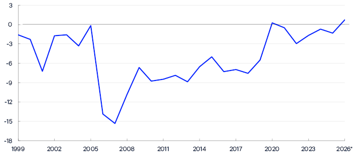
Net financial investment shows the difference between households’ financial investment and borrowing and is a measure of households’ financial saving. Households’ borrowing has generally been higher than financial saving and hence led to negative net financial investment (Chart 2.9).25 Households’ total net financial investment increased markedly during the pandemic before declining somewhat again. The rise was driven by higher household saving in bank deposits and securities. Over the past four quarters, net financial investment has been positive and equivalent to just below 1% of household disposable income. Higher interest rates may have contributed to this development by making it more attractive to save and less attractive to borrow. Greater uncertainty may also have given households an incentive to build up financial buffers.26
Net financial investment as a share of disposable income. Percent27
Households’ total holdings of bank deposits, listed equities and mutual fund units have increased more than debt since the pandemic (Chart 2.10). Both net financial investment and appreciation of securities have contributed to this development. The increase has been most pronounced for mutual fund units, partly reflecting rising equity prices. Over the past four quarters, households’ total liquid assets accounted for approximately 60% of total household debt.
Liquid assets as a share of debt. Four-quarter moving average28
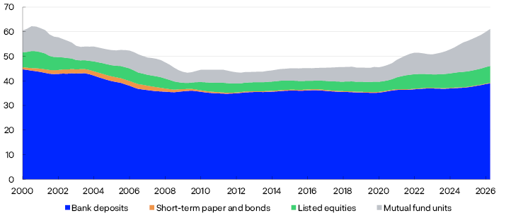
Valuation gains have made a substantial contribution to the rise in liquid buffers
As household financial buffers have increased and a large share is invested in mutual funds and listed equities, developments in financial markets can have a greater impact on the size of liquid buffers ahead. Developments in households’ financial asset holdings can be divided into contributions from active saving and value changes.
With the exception of 2022, the total stock of households’ mutual fund units and listed equities has increased relative to disposable income since the pandemic (Chart 2.11, left panel). Some of the increase is due to households’ net purchase of fund units and equities, ie active saving.29 However, the largest contribution to the increase came from changes in the value of existing financial assets.30 The contribution from value changes was particularly large in 2024 but also considerable in 2025.31 Over the past four quarters, households’ holdings of mutual fund units and listed equities have increased by an amount equivalent to just over 9% of disposable income. Approximately 70% of this increase is due to value changes.
Change in holdings as a share of disposable income. Percent32
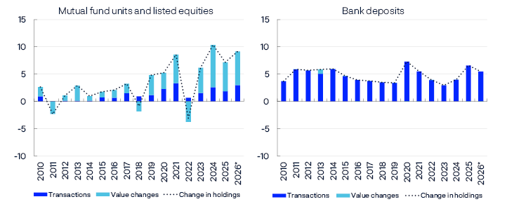
By comparison, households’ overall active saving in bank deposits declined relative to disposable income after the pandemic but has risen again since 2023 (Chart 2.11, right panel). The rise was particularly pronounced in 2025. Over the past four quarters, the increase in bank deposits accounted for slightly more than 5% of households’ disposable income.
More households have a more diversified financial portfolio
Household resilience depends not only on overall financial buffers but also on their distribution across households. Microdata are therefore used to examine more closely how the buffers have developed across households.
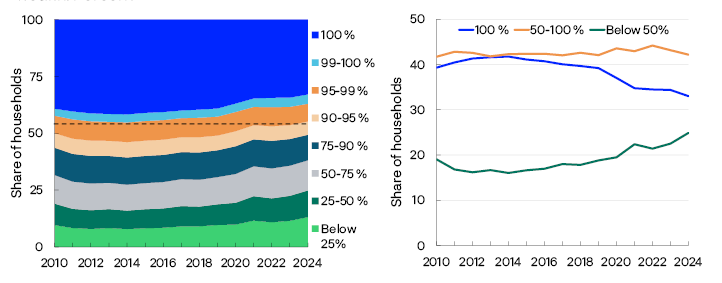
Bank deposits are the most liquid part of households’ accumulated savings and the dominant form of financial wealth for most households (Chart 2.12, left panel).33 Half of households hold more than 90% of their financial wealth in bank deposits, while just under one-third hold only bank deposits. At the same time, the share of households holding all their financial wealth in bank deposits has declined (Chart 2.12, right panel). Households’ financial wealth has become slightly more diversified in recent years as a result of more households saving in funds and other financial assets. Some of these investments, such as broad-based index funds, can be realised quickly to improve liquidity.
Share of households within different bank deposit intervals relative to share of financial wealth. Percent34
Households’ liquid buffers have increased more than income
For the median household, bank deposits accounted for slightly less than 30% of annual after-tax income in 2024 (Chart 2.13, left panel). After the marked rise during the pandemic, bank deposits rose more slowly than income across large parts of the distribution and in 2024 were approximately at the pre-pandemic level.Preliminary figures from tax assessments indicate, however, that bank deposits rose more than income across large parts of the distribution in 2025 (see orange bars in the chart).

If fund units and equity savings account balances are included in the liquid buffer measure, the level rises substantially (Chart 2.13, right panel).36 With this broader measure, liquid buffers increased again in 2024, despite the decline in bank deposits as a share of income. In 2024, the median household’s liquid buffer was equivalent to more than 40% of annual after-tax income, higher than in the pre-pandemic period.
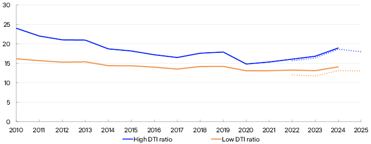
At the same time, some households have small liquid buffers. In 2024, approximately 19% of households with DTI ratios above three times after-tax income had little or no liquid buffer in the form of bank deposits (Chart 2.14). The share increased somewhat from 2023, but was approximately at the pre-pandemic level. Preliminary figures from tax assessments indicate that the share declined somewhat in 2025.
Share of households with bank deposits lower than half a month’s net pay. Percent37
25 In Statistics Norway’s Financial accounts by sector, saving in collective pension schemes is included in net financial investment. Since these are illiquid assets, they are excluded from this analysis.
26 Opinion’s Forbrukermeter [consumer meter] (in Norwegian only) and Finance Norway’s Forventningsbarometer [expectations barometer] (in Norwegian only) show that Norwegians’ confidence in their own financial situation and in the Norwegian economy is still lower than before inflation picked up and interest rates rose.
27 Period: 1999–2026 Q2.
Households’ net financial investment shows financial investment less borrowing. Collective pension liabilities are excluded from households’ financial investment.
* 2026 shows the sum of net financial investment over the latest four quarters for which data are available, from 2025 Q3 to 2026 Q2, measured as a share of disposable income.
28 Period: 2000 Q1–2026 Q2.
Households’ holdings of selected liquid financial assets as a share of total debt.
29 Shown in Chart 2.11 by transactions.
30 In Statistics Norway’s financial accounts by sector, this is referred to as andre endringer [other changes] that are not due to transactions. For securities, this primarily reflects appreciation, depreciation and exchange rate movements, but can also be due to changes in financial market classification and structure.
31 There is more uncertainty than normal related to the data underlying mutual fund unit transactions from 2025. This is due to structural changes in Statistics Norway’ underlying data, with a number of major fund managers having moved their portfolios abroad.
32 Period: 2010–2026 Q2.
Transactions are net investments by households in financial claims. Value changes include, among other things, value changes resulting from price and exchange rate changes, as well as changes in classification and structure in financial markets.
* 2026 shows the sum of transactions and other changes over the latest four quarters for which data are available, from 2025 Q3 to 2026 Q2, measured as a share of disposable income.
33 Underlying data are for 2024 because the figures for financial wealth from the Norwegian Tax Administration for 2025 are not processed in the same way as the income and wealth statistics from Statistics Norway.
34 Left panel:
Period: 2010–2024.
The shares are stacked and sum up to 100%. The broken line at 50% specifies the median in the distribution.
Right panel:
Period: 2010–2024.
The shares are shown separately and are not stacked.
In both panels, households whose main income earner is under 25, over 90 or self-employed are excluded, as are households in the top percentile of net wealth distribution.
35 Left panel:
Period: 2010–2025.
Right panel:
Period: 2010–2024
Liquid assets are defined as bank deposits, equity savings accounts and mutual funds.
In both panels, households whose main income earner is under 25, over 90 or self-employed are excluded. Households in the top percentile of net wealth distribution are also excluded.
The box plots show the 10th, 25th, 50th, 75th and 90th percentiles (indicated by the lower horizontal line on the black vertical line, the bottom of the blue box, the diamond, the top of the blue box and the upper horizontal line on the black vertical line, respectively).
* Figures for 2022–2025 are estimates generated from tax assessment data based on household composition in the previous year.
36 The data extend to 2024 because the 2025 figures for mutual funds and equity savings accounts from the Norwegian Tax Administration have not been processed in the same way as Statistics Norway’s income and wealth statistics.
37 Period: 2010–2025.
DTI ratio is debt as a share of after-tax income.
A low DTI ratio is below 300%. A high DTI ratio is above 300%. Households whose main income earner is under 25, over 90 or self-employed are excluded. Households in the top percentile of net wealth distribution are also excluded. The broken lines show figures from tax assessment data and are estimates based on household composition from the previous year.
2.4 House price inflation has declined despite low residential construction
The housing market is key to the assessment of financial stability, partly due to the interplay between house prices and debt.38 Housing is a key asset for households and an important reason why they take on substantial debt.
For a long time, house prices increased faster than household income (Chart 2.15). This increased household sector vulnerability as household DTI ratios increased at the same time (Chart 2.1). In recent years, house prices relative to disposable income have declined. Following a period of moderate house price inflation and high turnover in the secondary housing market in autumn 2025, house price inflation has slowed and remained low in 2026. Low house price inflation so far in 2026 has coincided with household credit growth levelling off (Chart 2.3, right panel). At the same time, there are wide regional differences. House price inflation has recently been particularly weak in the Oslo area, but high in other cities in Norway. Annual house price inflation is expected to be a bit lower in 2026 and 2027 than in 2025, before picking up again in pace with an increase in housing investment (see Monetary Policy Report 3/2026).
House prices relative to per capita disposable income. Index. 1998 Q4 = 10039

When house prices increase faster than household income over time, fewer households may be able to purchase their own home. In recent years, alternative housing purchase models that reduce the need for accumulated equity have emerged, with rent-to-own and shared ownership being the most common. Rent-to-own combines renting with a right to subsequently purchase, while shared ownership involves buying a share of the home and renting the rest, often with the option of increasing the ownership share over time. Regulatory changes are currently under way to facilitate increased use of such models (see box below).
New legislation provides for new housing purchase models
The Norwegian Ministry of Local Government and Regional Development recently conducted a public consultation about new regulations for borettslag and sameier, the two main forms of housing cooperatives in Norway. The aim is to promote rent-to-own and shared ownership models in new housing projects. Under the proposal, model providers are permitted to own a larger share of homes in housing cooperatives than is the case today. At the same time, more detailed contractual requirements and special rules are proposed to safeguard consumer protection and the balance of power in housing companies and cooperatives.
Norges Bank has submitted a consultation response with some remarks on aspects of the housing purchase models that may have implications for systemic risk and financial stability. These models are currently assessed to have only minor implications for financial stability as their use is limited. However, the models may have greater significance if their use becomes more widespread or if financing becomes more concentrated. The rent-to-own and shared ownership models resemble financial service offerings and their structure may make them subject to licensing under the Financial Institutions Act. In Norges Bank’s assessment, further clarification is needed as to when providers of housing purchase models are engaged in activities subject to licensing and which regulatory requirements then apply. Such clarifications will contribute to equal regulatory treatment and set clearer parameters for housing purchase models.
Low residential construction is being offset by lower household formation and an ample stock of existing homes
House prices are determined by a range of factors, including interest rates, income and the tax policy stance. The housing supply also has implications for house prices over time. The relationship between the increase in the number of homes and household formation is an indicator of developments in housing market supply and demand. Residential construction has been outpaced by household formation since 2018 (Chart 2.16). The number of housing start permits and completions has fallen since 2022, partly owing to higher interest rates and increased costs.40 At the same time, household formation has slowed, particularly in 2025, in line with lower population growth. Slower household formation, combined with an increased supply of existing homes, may have contributed to weaker house price inflation in the secondary housing market, despite low residential construction.
Building permits and completions and annual change in the number of households. In thousands41
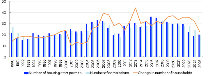
The extent to which household formation has outpaced the rise in the number of homes varies across regions in Norway. In the period between 2021 and 2024, household formation outpaced the number of dwellings in all urbanisation classes (Chart 2.17).42 In 2025, the difference increased further in the most urban areas outside Oslo and in urbanisation class 5. In the other urbanisation classes, the rise in the number of households and homes was approximately the same.
Rise in the number of dwellings and households by urbanisation class. Percent43

Over time, the difference has been widest in the most urban areas, which may have contributed to higher house prices there (Chart 2.18). At the same time, the difference is less pronounced in most areas than it has been in the post-pandemic years.
Rise in the number of dwellings and households by urbanisation class. Percent44
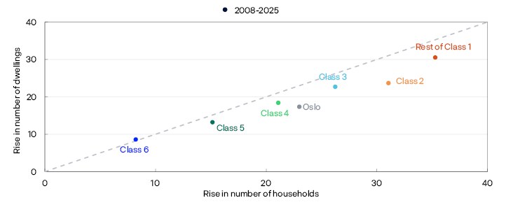
Data underlying the analyses in this section
The analyses of households are based on statistics that use tax returns as the most important data source. Tax returns include household-level information about income, debt and wealth.
For the period to end-2024, complete income and wealth statistics for Norwegian households from Statistics Norway are used. For charts containing figures from tax assessments, tax return data from the Norwegian Tax Administration available by 1 August 2026 is used the subsequent year ie after the income year. As tax returns do not include information on individuals’ household status, the previous year’s data on household composition from Statistics Norway’s income and wealth statistics are used to aggregate the variables up to household level.
38 Residential mortgage loans account for most household debt. Higher house prices raise the value of collateral and thus increase borrowing opportunities. Higher house prices may result in increased credit demand over time, and improved access to credit may result in higher house prices through increased housing demand.
39 Period: 1983 Q1–2026 Q2.
House prices relative to disposable income per capita, persons aged 15 to 74.
40 See Section 3.3 for a more detailed description of profitability and activity in the real estate development market.
41 Period: 1990–2025.
A building permit is issued by the municipality and gives a developer permission to start construction. The permit is valid for three years.
A housing completion is a dwelling that has either been granted a temporary use permit or a certificate of completion, or a completed building that is exempt from building application requirements but is nevertheless subject to notification and registered in the Land Register.
42 The chart compares the rise in the number of households with the rise in the number of homes. If these two growth rates are the same, the observations will lie on the red diagonal line. Observations to the right of the line indicate that the number of households has increased more than the number of homes, while observations to the left indicate the opposite.
43 Period: 2021–2025.
Statistics Norway’s urbanisation classes are based on access to workplaces and services. A higher class indicates lower urbanisation.
44 Period: 2008–2025.
Statistics Norway’s urbanisation classes are based on access to workplaces and services. A higher class indicates lower urbanisation.
A historical perspective on household debt-servicing capacity
Norwegian households have high debt-to-income (DTI) ratios, and this high debt is a key vulnerability in the Norwegian financial system. For a long period, debt rose faster than income. At the same time, the default rate has remained low over the past 25 years, irrespective of business cycles. Developments in households’ debt must therefore be viewed in the light of developments in their debt-servicing capacity.
A new analysis examines developments in household debt-servicing capacity over time.1 The analysis uses household-level microdata to shed light on developments in debt-servicing capacity in the period between 2001 and 2024. The analysis focuses on homeowners since they hold most of the debt among Norwegian households. The amount of debt households can service depends, among other things, on income, consumer expenditure, housing costs and interest rate levels. To assess how household debt-servicing capacity has evolved, developments in these components are examined first.
Debt-servicing income has increased markedly
The portion of income that can be used for debt servicing, in the form of both interest and principal payments, is referred to as debt-servicing income, ie income after tax and necessary expenditure on ordinary consumption and housing costs.
As a measure of households’ ordinary consumer expenditure, the Consumption Research Norway (SIFO) Reference Budget is used, which provides estimates of expenditure on a modest level of consumption for different types of households. These expenditures declined as a share of after-tax income through the 2000s, before levelling off somewhat (Chart 2.A, left panel). For the median household, the share fell from just over 50% in 2001 to just under 40% in 2024.
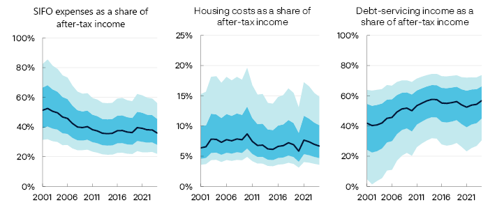
Meanwhile, housing costs have been relatively stable compared to income, accounting for around 7% of after-tax income for the median household through much of the period (Chart 2.A, middle panel). The National Federation of House Owners in Norway (Huseierne) Housing Cost Index is used as a measure of these costs.3
For the median household, debt-servicing income increased from around 40% of after-tax income in 2001 to around 55% in 2024 (Chart 2.A, right panel). There was a substantial increase in the period to 2015. This share then levelled off, before falling somewhat around the pandemic period. Since 2022, the share has risen again, primarily reflecting higher income.
Lower interest rates have eased the burden of higher debt
The increase in the debt-to-income (DTI) ratio over the past 25 years must also be seen in light of interest rate developments. Through much of the period, interest rates declined. Lower interest rates eased the burden of increased borrowing and contributed to more stable developments in interest burdens, measured as interest expenses as a share of after-tax income. In recent years, interest burdens have increased considerably in pace with higher interest rates.
Households’ discretionary income has also increased over time
When interest expenses are deducted from debt-servicing income, what remains is households’ discretionary income. This income can be used for savings, principal payments and consumption beyond what has been assumed in this analysis.
In line with the increase in debt-servicing income and a relatively stable interest burden, discretionary income has increased as a share of after-tax income. For the median household, discretionary income rose from around 30% of after-tax income in 2001 to almost 50% in 2015 (Chart 2.B, left panel), before levelling off and declining to just over 40% in 2024. The full distribution was shifted towards higher levels for discretionary income in 2024 compared with 2001.
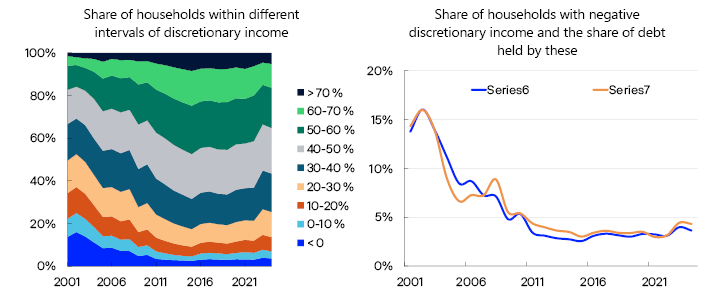
From a financial stability perspective, developments in the share of households with low or negative discretionary income are of particular interest, as these households have limited capacity to cope with economic downturns. The share of households with negative discretionary income fell markedly through the 2000s and has since remained at a relatively low level (Chart 2.B, right panel). The share of total debt held by households with negative discretionary income has also fallen considerably. Compared with levels in the 2000s, the increase in the share of households with negative discretionary income in 2023 and 2024, owing to higher interest rates and inflation, was moderate.
Households’ debt burdens have increased less measured against debt-servicing income
The increase in debt-servicing income has given households the opportunity to either increase consumption beyond an ordinary level or service more debt. These developments have implications for the interpretation of households’ debt burdens.
The traditional measure of debt burden assesses households’ debt relative to income.5 A supplementary measure is debt as a share of debt-servicing income since this is the share of income available for debt servicing.
Chart 2.C shows how developments in households’ debt burden depend on the income measure used. Measured relative to after-tax income, the median household debt burden more than doubled between 2001 and 2020, before declining somewhat in the subsequent years. Measured relative to debt-servicing income, the debt burden has increased markedly less.
Median. Index, 2001 = 1006

Norwegian households’ strong debt-servicing capacity is well documented in previous analyses.7 What is new in this analysis is the long period over which developments are tracked and the examination of how improved debt-servicing capacity has helped households service ever-higher debt while defaults have remained low.
1 See Ellingsen, J., K.-G. Lindquist and B.H. Vatne (2026), “Et historisk blikk på husholdningenes gjeldsbetjeningsevne” [A historical perspective on household debt-servicing capacity] (Forthcoming in English). Staff Memo 6/2026. Norges Bank.
2 Period: 2001–2024.
The sample only includes homeowners.
Households whose main income earner is under 25, over 90 or self-employed are excluded.
SIFO expenses are based on household size and the SIFO reference budget.
Housing costs are based on the National Federation of House Owners in Norway (Huseierne) Housing Cost Index and include property tax, municipal charges, energy and insurance for a 120-square-metre dwelling.
Debt-servicing income is defined as after-tax income less SIFO expenses and housing costs.
3 The index comprises property tax, municipal charges and costs related to energy, insurance and maintenance, as well as interest expenses. In the analysis, maintenance is excluded, and observed interest expenses from the microdata are included as a separate expense component.
4 Period: 2001–2024.
The sample only includes homeowners.
Households whose main income earner is under 25, over 90 or self-employed are excluded.
Discretionary income is defined as after-tax income less SIFO expenses, housing expenses and interest expenses.
SIFO expenses are based on household size and the SIFO reference budget.
Housing costs are based on the National Federation of House Owners in Norway (Huseierne) Housing Cost Index and include property tax, municipal charges, energy and insurance for a 120-square-metre dwelling.
5 Gross income, after-tax income and disposable income are all commonly used as income measures when calculating debt burden.
6 Period: 2001–2024.
The sample only includes homeowners.
Households whose main income earner is under 25, over 90 or self-employed are excluded.
Debt-servicing income is defined as after-tax income less SIFO expenses and housing expenses.
SIFO expenses are based on household size and the SIFO reference budget. Housing costs are based on the National Federation of House Owners in Norway (Huseierne) Housing Cost Index and include property tax, municipal charges, energy and insurance for a 120-square-metre dwelling.
7 See eg Lindquist, K.-G., H. Solheim and B.H. Vatne (2022) “Norwegian homeowners’ debt-servicing capacity is adequate”. Staff Memo 8/2022. Norges Bank.
3.1 Overall, Norwegian firms are financially sound
Financial positions in the Norwegian corporate sector were stable through 2025.1 Annual financial statements show that corporate profitability2 improved, while solvency was broadly unchanged. According to Norges Bank’s Regional Network, profitability has changed little so far in 2026 and moderate activity growth is expected ahead (see Regional Network 3/2026). Strengthened household purchasing power, increased defence spending and data centre buildout are contributing to the upturn, while low construction activity is having a dampening effect. The increase in bank and bond debt was low through 2025, and corporate solvency is strong overall. Annual financial statements show that equity ratios increased in most sectors in 2025 (Chart 3.1).
Equity ratio all industries. Percent3
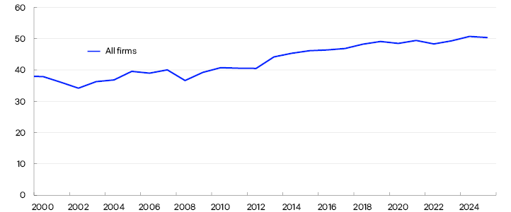
Profitability, as measured by firms’ operating margins, improved in 2025 (Chart 3.2). For sectors with high debt-to-income (DTI) ratios, such as real estate development and commercial real estate (CRE), interest expenses have reduced profitability considerably since 2022. Adjusted for interest expenses, operating margins in real estate development improved somewhat in 2025. Despite persistently low activity, profitability in construction improved in the period between 2024 and 2025, and operating margins after interest expenses are now in line with the historical average.
Operating margins before and after net interest expenses. Percent4
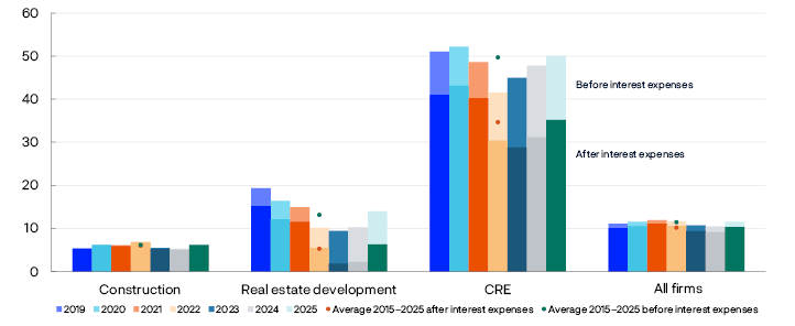
The real estate sector’s importance for financial stability
The financial position of real estate firms is important for financial stability because problems in these firms can result in bank losses. Historically, banks’ losses have been higher on loans to the corporate sector than to households.
CRE and real estate development loans amount to more than half of Norwegian banks’ total corporate exposures (Chart 3.A). Construction firms account for a smaller share of banks’ corporate exposures but a higher share of those employed in real estate.
Banks' lending to Norwegian non-financial firms as of September 2026. Percent
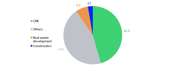
In a construction project, real estate developers normally own the project and take out loans secured on the project. Before providing financing, Banks normally require either that a substantial share of the project is pre-sold or that binding lease agreements have been made. The contractor and sub-contractors are responsible for the building construction.
When a building is completed, ownership is normally handed over to a household if the property is residential or to a CRE firm if it is commercial. The new building usually becomes a part of the CRE firm’s existing portfolio of commercial rental properties. Banks play a key role in financing building purchases, both for households and CRE firms. For CRE firms, banks also play a key role in refinancing loans.
Banks’ credit risk on exposures to real estate developers and CRE is closely linked to price developments in the real estate market. For real estate development exposures, the risk also reflects demand for new commercial and residential buildings, and the number of unsold units in projects that have already been started.
1 The financial statement analysis covers Norwegian non-financial limited companies that have submitted annual financial statements for the applicable year. Firms in oil and gas extraction and power companies are omitted from the analysis owing to substantial earnings volatility that has a disproportionately large impact on overall developments. Banks’ exposures to such firms are relatively small.
2 Measured as EBITDA/revenue and (EBITDA-net interest expenses)/revenue.
3 Period: 2000–2025.
Equity ratio is book equity as a share of total capital (equity and debt).
4 Period: 2019–2025.
Operating margins before interest expenses are earnings (EBITDA) as a share of revenue. Operating margins after interest expenses are earnings (EBITDA) minus interest expenses plus interest income, as a share of revenue.
Net interest expenses are shown by the light shaded areas of the bars.
3.2 Higher rate of bankruptcies in real estate development
Weaker economic developments contributed to a gradual increase in the share of bankruptcies among Norwegian firms through 2023 and 2024. At the same time, the increase reflects a normalisation following unusually low bankruptcy figures during the pandemic. So far in 2026, the corporate bankruptcy rate has been relatively stable and broadly in line with the average for the past 10 years (see broken line in Chart 3.3, left panel).5
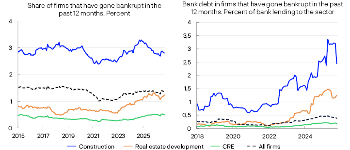
Higher interest expenses and low construction activity have markedly increased the bankruptcy rate in the real estate sector in recent years. The rise has been most pronounced in real estate development, where the bankruptcy rate has more than doubled since 2022. The firms that have gone bankrupt are primarily individual stand-alone project companies of a limited size.7 Bank debt has also risen among bankrupt real estate developers (Chart 3.3, right panel). Over the past 12 months, the overall bank debt of bankrupt real estate developers has amounted to NOK 1.9bn, approximately ten times more than the average in the years preceding the rise in bankruptcies. The six largest bankruptcies account for about 60% of the bank debt of real estate developers that went bankrupt over the past 12 months.8 In CRE, the bankruptcy rate has risen less. Nevertheless, the bank debt of bankrupt CRE firms has increased in recent years. Measured as banks’ total CRE exposure, the extent is limited.
The bankruptcy rate is normally higher in construction, as contractors often have small margins, which makes them more vulnerable to a decline in demand or sudden cost increases. However, debt in the construction sector is limited.
Developments in debt collection cases indicate a slight decline in bankruptcies in 2027
Payment remarks may provide an early indication of payment difficulties. In recent years, among the firms with at least one outstanding debt collection case at the end of a given month, around 10% went bankrupt within a year. Norges Bank’s analyses find that firms with four or more outstanding debt collection cases are around four times as likely to go bankrupt within one year as firms with one to three such cases.9 Debt collection cases may therefore provide early information about credit risk before problems become evident in default rates. If many firms face payment difficulties at the same time, an increase in defaults and credit losses could reduce banks’ profitability and capacity to lend.
The share of firms with debt collection cases increased steadily after the pandemic but has levelled off over the past two years. A simple, stylised model10 for developments in the share of bankruptcies one year ahead, based on the share of firms with debt collection cases, indicates that the share of bankruptcies will remain broadly unchanged in 2027, close to 1.2% (Chart 3.4). This is broadly in line with the average share of bankruptcies over the past ten years excluding the pandemic period.
Actual and predicted bankruptcy rate within one year. Percent11
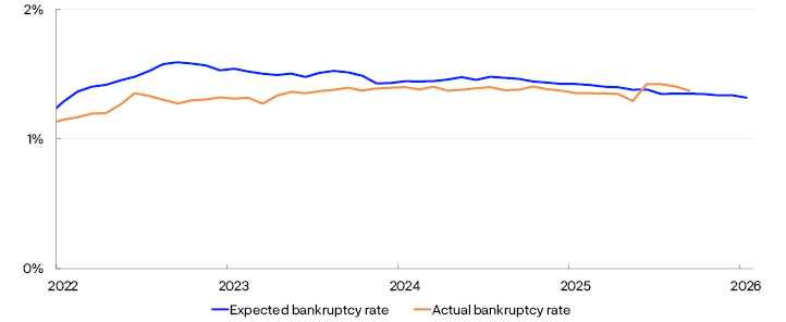
Sources: Brønnøysund Register Centre, Dun & Bradstreet and Norges Bank Norges Bank’s bankruptcy probability model, KOSMO, complements this picture (Chart 3.5). The model estimates the probability of a firm going bankrupt within one year, based on accounting data and payment remarks from the previous year, as well as macroeconomic indicators for the current year. When weighted by bank debt, the bankruptcy probability has increased from a low level after the pandemic and is now higher than before the rise in interest rates. The model indicates broadly unchanged bankruptcy risk ahead for the sectors as a whole, but developments vary across sectors. Risk is expected to increase in real estate and construction, with the former accounting for a growing share of overall bankruptcy risk owing to its large share of bank debt.12
Debt-weighted bankruptcy probability and bankruptcy debt. Percent13
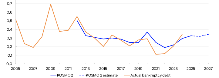
5 In most sectors, the bankruptcy rate increased markedly in June, primarily reflecting a rise in compulsory liquidations. Virtually all firms that were subject to compulsory liquidation in June were alerted in March about dissolution as a consequence of failure to submit financial statements for 2024. In previous years, compulsory liquidations were distributed over several months. In 2026, a larger proportion was registered in June, contributing to the marked rise in that month. Firms that were subject to compulsory liquidation generally had little debt. The rise therefore does not reflect an underlying rise in credit risk.
6 Period: January 2015–October 2026 in the left panel and January 2019–October 2026 in the right panel.
Share of firms that have gone bankrupt in the past 12 months is the sum of bankruptcies in the past 12 months as a share of the number of firms in the sector in the past 12 months.
Bank debt in firms that have gone bankrupt has been obtained from the firms’ most recently published annual accounts and are not equivalent to banks’ actual credit losses. Bankruptcies comprise both opening of bankruptcy proceedings and compulsory liquidations.
7 Of the 190 real estate developers that went bankrupt in the past 12 months, 84% had no employees.
8 Only a third of the firms that went bankrupt in the past 12 month had bank debt. The largest of them was Nøstad Brygge AS, a residential project that went bankrupt in 2026 with NOK 0.6bn in bank debt according to its last submitted financial statements, approximately a third of ’total bank debt of bankrupt real estate developers. Other notable bankruptcies include Nordbolig Innlandet AS, Velbygd Østlandet AS and Chistiania Eiendomsselskab AS, whose respective debt amounted to between NOK 95 and 156m. Figures for bank debt are obtained from firms’ last submitted financial statements and are not the same as banks’ actual losses.
9 See Hjelseth, I.N. and K. Liaudinskas (2024) “Record Increase in Payment Remarks: A Red Flag for Norwegian Firms?”. Staff Memo 9/2024. Norges Bank.
10 The model estimates the number of bankruptcies over the next 12 months based on the number of firms with at least one outstanding debt collection case, the historical share of these firms that have gone bankrupt within the following year, and the share of bankruptcies that do not receive payment remarks. See Hjelseth, I.N. and K. Liaudinskas (2024) “Record Increase in Payment Remarks: A Red Flag for Norwegian Firms?”. Staff Memo 9/2024. Norges Bank.
11 Period: January 2022–October 2026.
The bankruptcy rate in the past 12 months is the sum of bankruptcies over the past 12 months as a share of the number of firms over the past 12 months.
The predicted bankruptcy rate is calculated from the share of firms that go bankrupt within one year after at least one debt collection case (12-month moving average) and the share of firms that go bankrupt without having had any debt collection cases in the past year (12-month moving average).
12 The projections for 2026 and 2027 are partly based on macroeconomic projections and may change when more firms have submitted their 2025 financial statements. Hjelseth, I.N., K. Liaudinskas and S.K. Thuve (2024) “New microdata for loan defaults provide better estimates of banks’ credit losses”. Staff Memo 10/2024. Norges Bank.
13 Period: 2005–2027.
Debt-weighted bankruptcy probability is estimated using Norges Bank’s bankruptcy probability model KOSMO, where firms’ bankruptcy probability is weighted using bank debt.
Bankruptcy debt is bank debt in bankrupt firms as a share of total bank debt. Projections for 2026 and 2027.
3.3 Low construction activity remains a challenge for real estate developers
High construction and financing costs have dampened demand for new residential and commercial property in recent years. Both new home sales and housing start permits have remained at a low level so far in 2026 (Chart 3.6). Real estate developers are particularly vulnerable as they bear a large share of project and financing risk, and many are highly indebted (see “The real estate sector’s importance for financial stability”). Lending to real estate development accounts for approximately 7% of banks’ Norwegian corporate exposures.
Number of homes. Sum past 12 months14
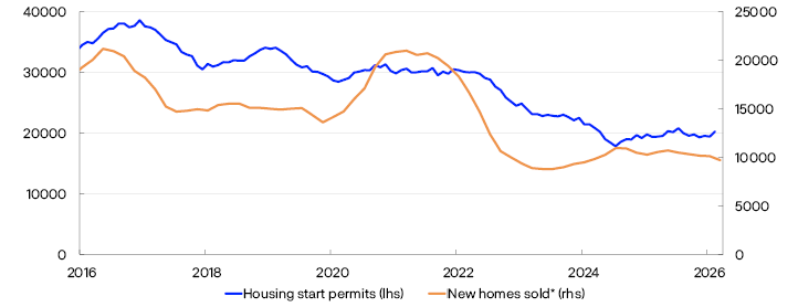
The profitability of real estate development projects is under pressure on both the demand and cost sides. In addition to high construction and financing costs, market participants point to increased costs associated with sequencing requirements15 and lengthy planning processes. Sequencing requirements further reduce profitability when margins are already under pressure, while high interest rates increase the cost of lengthy planning processes. The price differential between new and existing homes has therefore widened considerably, which makes new homes relatively less attractive, while high costs limit developers’ scope for reducing prices. At the same time, a large supply of existing homes and lower household growth have contributed to weak price developments in secondary housing market segments (see further discussion in Section 2.4). This limits buyers’ willingness to pay for new homes.
For many housing projects, expected sales revenues are therefore insufficient to cover costs and investors’ required rate of return. Lower land value is a possible adjustment that could make projects financially viable. Norges Bank’s analyses indicate, however, that land-related values remain elevated and are historically high (see “Land accounts for a larger share of residential property values”).
Weak project finances are an important reason why activity remains low. Most developers depend on external financing from banks that normally require a 50% pre-sale rate. Owing to weak new home sales, fewer projects are securing sufficient pre-sales to obtain financing and proceed to construction. Norges Bank’s Regional Network contacts report few new residential and commercial construction projects so far in 2026. Activity remains low in most regions. South-West Norway is an exception, where residential construction has increased, partly reflect spillovers from high activity related to energy production. In parts of the region, house prices have also risen considerably more than the national average over the past year.
Improved profitability and interest coverage ratio despite low activity
The financial position of real estate developers improved somewhat in 2025, after having deteriorated markedly in the preceding years. In the period between 2021 and 2024, interest expenses doubled while earnings were almost halved (Chart 3.7, left panel). This led to a marked decline in the interest coverage ratio (ICR) (Chart 3.7, right panel). Profitability improved in 2025 despite continued low activity. Costs fell more than revenues and, together with lower interest expenses, contributed to a slight increase in the ICR, from around 1 in 2023 and 2024, when earnings barely covered interest expenses, to 1.2 in 2025.
EBITDA and interest expenses. Indexed. 2019 = 100. Interest coverage ratio (ICR)16

The higher ICR largely reflects firms’ adjustment to the low level of activity, but the improvement is not broad-based. Nearly 30% of firms with interest expenses and positive earnings had an ICR below 1 in 2025, broadly unchanged from 2023 (Chart 3.8, left panel).
Distribution by interest coverage ratio and equity ratio. Share of firms. Percent17

Real estate developers’ solvency has also strengthened over the past two years. Debt and assets have declined amid lower activity and fewer project starts, while a small number of large firms have received capital injections from their owners. Overall, this has contributed to a marked increase in equity ratios. Lower debt and a higher equity ratio leave firms as a whole better able to absorb losses and withstand high financing costs. At the same time, the share of firms with negative equity has risen further, to 26% (Chart 3.8, right panel). Some of these firms will likely be wound up or go bankrupt. Real estate developers that have gone bankrupt have generally had negative or very low equity in their most recently submitted financial statements.
For the sector as a whole, the ICR is expected to remain broadly unchanged in 2026 and 2027, although differences across firms are considerable. The projections assume that interest rates follow the path projected in Monetary Policy Report 3/2026 and that debt in the sector remains unchanged. The policy rate has been raised in 2026, but as it was lowered over the course of 2025, the average interest rate this year will be broadly unchanged from last year. With unchanged debt levels, interest expenses will therefore also remain broadly unchanged in 2026. In 2027, higher interest rates will feed fully through to annual interest expenses, but this will be offset to a large extent by higher revenues as construction activity is expected to pick up somewhat. The projections largely depend on construction activity. A number of contacts in Norges Bank’s Regional Network report that residential construction has troughed, but many report that the recovery continues to be delayed. In a downside scenario where residential investment falls further instead of picking up, the ICR for the sector as a whole would decline to 0.9 in 2027. Earnings would then be insufficient to cover interest expenses, and more firms than today would need to draw on their financial buffers.
14 Period: January 2016–October 2026. Housing start data up to and including September 2026.
* Includes homes in projects of more than 15 units. Statistics frequency has been converted from 12-month to one-month with equal distribution.
15 Sequencing requirements are provisions in land-use plans governing the order of developments. Such requirements may include completion of certain infrastructure developments before construction can commence or buildings can be commissioned.
16 Period: 2016–2025 (left panel) and 2000–2027 (right panel). Projections for 2026 and 2027 from FSR 2026 H2.
Interest coverage ratio is total earnings (EBITDA) as a share of total interest expenses for legal entities in real estate development.
The left panel shows total EBITDA and total interest expenses for the same units, indexed to 2019 = 100. In the FSR 2026 H2 projections, the average interest rate is assumed to decrease by 0.06 percentage point in 2026 and increase by 0.3 percentage point in 2027, in line with the policy rate path in Monetary Policy Report 3/2026. Furthermore, operating income is assumed to follow housing investment and increase by 0.3% in 2026 and 2.7% in 2027, while operating costs are assumed to increase by 0.3% in 2026 and 2.5% in 2027. Interest-bearing debt is assumed to remain unchanged. In the downside scenario, housing investment is assumed to decrease further, so that operating income falls by 3.5% in 2026 and 11.3% in 2027, while operating costs fall by 3.1% in 2026 and 10.1% in 2027. Interest rates and interest-bearing debt are assumed develop as in the baseline scenario.
17 Period: 2020, 2023 and 2025.
The left panel includes all firms in the sector. The right panel includes all firms with interest expenses and positive earnings.
Land accounts for a larger share of residential property values
Land value is one of several components in a real estate developer’s project calculation (Chart 3.B).1 On the revenue side are expected sales revenues, which must cover the development costs related to the land, the construction of the residential property, financing during the construction period and other development costs. In addition, the developer’s margin on the project must be sufficient. If expected sales revenue is insufficient to cover costs and provide this margin, the project may be postponed or abandoned. Lower land value is one possible adjustment that could make a project financially viable. In a new analysis, developments in land-related values for flats in Oslo are examined in the period between 2003 and 2025.2
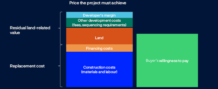
Source: Norges Bank Land value is difficult to measure. When an existing home is sold, the market price of the property as a whole is observed. This price reflects the value of the building itself, the land and other development-related components. Such components can be estimated, for example in a valuation but are not observed separately in the market transaction. There are also few directly comparable land transactions. The analysis focuses on flats in Oslo. The land-related value of a residential property is estimated indirectly, ie as the difference between the observed price of the existing property and its estimated replacement cost.4 The land-related value is therefore a residual measure that can also capture other development costs such as those related to planning and regulatory requirements, as well as the developer’s margin.
Replacement cost is calculated as the sum of construction contract costs and financing costs during the construction period (Chart 3.B). Construction contract costs are projected based on costs per square metre for a reference building from the 2025 Norsk Prisbok [a construction cost reference guide]. The costs are estimated retroactively using Statistics Norway’s construction cost index and are adjusted for developments in productivity. For existing homes, replacement cost is also adjusted for depreciation with age. This adjustment is based on the relationship between age and prices of flats sold in Oslo, controlling for eg attributes and location.5
Chart 3.C (left panel) shows price developments in the existing housing market, estimated replacement costs and land-related values for flats in Oslo since 2003. The calculations indicate that land-related value in the secondary market has increased considerably and fluctuated markedly more than replacement costs. Developments in replacement costs have been far more stable than residential property prices, and much of the variation in the prices is therefore reflected in the land-related value. Studies from the US also find that over time land values have increased considerably and fluctuated more than building values.6 The estimated land value fell during the financial crisis, rose sharply towards 2017 and reached a new peak around 2021. It has since fallen back somewhat but is still high from a historical perspective. One possible explanation for the strong growth is that housing demand in attractive areas has increased faster than the supply of development-ready land. Limited land area and time-consuming planning processes may have been contributing factors. If landowners also chose to postpone the sale or development of land sites in expectation of higher values later, supply may have been constrained further.
Oslo. Indices in real terms. 2003 Q4 = 1007
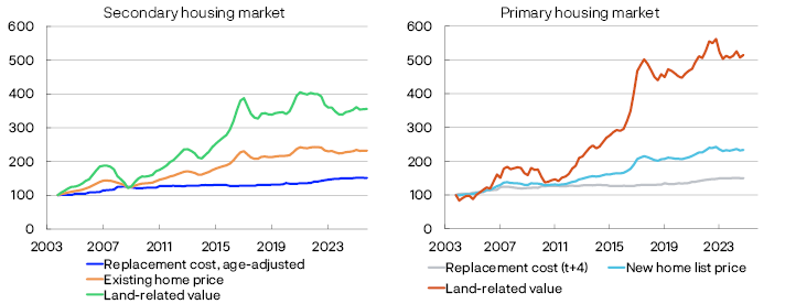
A corresponding estimate is also made for the primary housing market (Chart 3.C, right panel). A hedonic list price index for new homes is used.8 The estimate differs from that for the secondary market as replacement costs are not adjusted for age, and replacement costs four quarters ahead are used to account for the time between sales start and completion. As in the secondary market, land-related value in the primary market has also increased considerably and fluctuated markedly more than replacement costs. As the estimates are based on different homes and land sites, the comparison focuses on developments over time rather than on the levels of land-related values.
The estimates also suggest that land-related values in the primary and secondary markets followed broadly similar paths until 2016. Following the rise in house prices up to 2017, the rise in prices in the secondary housing market slowed markedly, while construction costs continued to rise. This pulled down the estimated land-related value in the secondary housing market (Chart 3.D). In the primary market, on the other hand, list prices continued to rise for some time, and the estimated land-related value therefore remained higher. The introduction of the DTI requirement in 2017 may have dampened housing demand and house prices and thereby contributed to weaker developments in land-related values in the secondary housing market, but higher construction costs or other conditions also may have contributed.


Period: 2003 Q4–2025 Q4. The series based on new home list prices ends in 2024 Q4. Both series are calculated in NOK per square metre and deflated by the CPI before they are indexed to 2003 Q4 = 100. The series are indexed separately and therefore show differences in developments rather than in levels for the land-related values.
See the tooltip to Chart 3.B for a more detailed description of the calculations.
Oslo. Indices in real terms. 2003 Q4 = 1009

The difference in the estimated land-related values has persisted in the years since 2017. From 2017 Q1 to 2024 Q4, real list prices for new homes rose by around 13%, while existing home prices were broadly unchanged. New home prices have therefore risen relative to existing home prices, which is also reflected in estimated land-related values. Land-related value based on new home list prices has remained elevated, while the value estimated based on existing home prices has been weaker. At the same time, new home sales have been weak in recent years and housing starts have been low.
Developments in the years since 2017 may partly reflect the fact that new home prices adjust more slowly than existing home prices when the market weakens.10 The secondary housing market is larger and more liquid, and prices are usually determined through bidding rounds. New homes are normally sold at list prices set by the developers. Real estate developers can be reluctant to reduce list prices if this entails loss realisation and weakens the financial outcome. Weaker demand may therefore result to a greater extent in fewer sales and postponed construction rather than lower list prices.
The estimates are also used to project the share of the estimated value of a new home that can be attributed to land-related values (Chart 3.E). The share is calculated as the land-related value from the secondary housing market divided by the sum of this value and the replacement cost of a new home. The results suggest that this share has increased from around one-third in 2003 to somewhat more than one-half at the end of 2025. Since 2017, the share has declined somewhat, since the replacement cost has increased while land-related values have remained fairly stable. Overall, the estimates suggest that a larger share of housing values is now attributable to the land-related component, which has also fluctuated considerably more than the replacement cost.
Estimated land-related value share of new builds in Oslo. Percent11
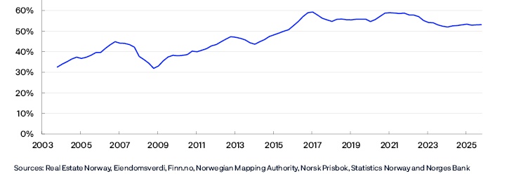
These developments have implications for financial stability. A high land-related value is not necessarily a vulnerability in itself. However, when the land-related component accounts for a larger share of the residential property value and has historically fluctuated more than construction costs (Chart 3.C), a decline in land-related values may have a greater impact on house prices and collateral values. The difference can be illustrated with a numerical example: if land-related values fall by 30%, the estimated housing value will fall by approximately 16% when the land share is just over half and the replacement cost remains unchanged. With a land share of one-third, the fall in value is only around 10%. Larger falls in housing values could reduce the equity buffers of highly leveraged households and, in the event of default, increase banks’ losses. For developers, the land-related value can be a large and particularly variable component of project viability, making the profitability of new projects sensitive to fluctuations in the housing market.
1 This box focuses on residential property and residential property projects, but the mechanisms described apply to real estate projects in general.
2 See Iden, Nenov and Plaku (2026), “Inferring Land Values in Oslo”, Norges Bank Staff Memo 7/2026, for a further discussion of the underlying data, methodology, results and robustness checks.
3 The chart shows the cost components of a residential property project relative to the buyer’s willingness to pay. In the example, the buyer’s willingness to pay is lower than the price required to cover the project costs and the required rate of return. The height of the bars and the distribution between the components are only illustrative and not based on actual data.
4 The methodology builds on the residual approach in Davis, M.A. and J. Heathcote (2007), “The price and quantity of residential land in the United States”, Journal of Monetary Economics, 54(8), pp 2595–2620.
5 The adjustment for age-related depreciation is based on the median age of flats sold in Oslo, which is 29 years. The median is calculated using transaction data for the latest available year (2021), and the deduction is held constant over time.
6 See eg Davis, M.A. and J. Heathcote (2007), “The Price and Quantity of Residential Land in the United States”, Journal of Monetary Economics, 54(8), pp 2595–2620. Davis, M.A. and M.G. Palumbo (2008): “The Price of Residential Land in Large US Cities”, Journal of Urban Economics, 63(1), pp 352–384.
7 Period: 2003 Q4–2025 Q4. Right panel ends at 2024 Q4. All series are calculated in NOK per square metre, deflated by CPI and then indexed. The indices show developments over time rather than differences in levels between the primary and secondary housing markets.
Left panel: Replacement cost is the construction cost of building an equivalent new residential property, including financing costs during the construction period and adjusted for age. Existing home price is the 2025 price per square metre of flats in Oslo, extended backwards using a quality-adjusted price index for all home types in Oslo. Land-related value is existing home price less replacement cost.
Right panel: Replacement cost (t+4) is the construction cost of building a new home, including financing costs during the construction period, four quarters ahead. This takes into account the fact that new homes are often sold before they are built. New home list price is the 2025 price per square metre of new flats in Oslo, extended backwards using Norges Bank’s hedonic list price index for new homes in Oslo, see Iden et al. (2026). Land-related value is new home list price less replacement cost (t+4).
8 For a more detailed description of the estimate of the list price index for new homes, see Iden A.E., P. Nenov and S. Plaku (2026), “Price Rigidities in the Market for New Homes”, Working Paper 8/2026. Norges Bank.
9 Period: 2003 Q4–2025 Q4. The series based on new home list prices ends in 2024 Q4. Both series are calculated in NOK per square metre and deflated by the CPI before they are indexed to 2003 Q4 = 100. The series are indexed separately and therefore show differences in developments rather than in levels for the land-related values.
See the tooltip to Chart 3.B for a more detailed description of the calculations.
10 Iden A.E., P. Nenov and S. Plaku (2026): “Price Rigidities in the Market for New Homes”, Working Paper 8/2026. Norges Bank.
11 Period: 2003 Q4–2025 Q4. The chart shows how large a share of a calculated home value for new construction can be attributed to land-related values. The land-related share is calculated as land-related value in the secondary housing market (existing home price less age-adjusted replacement cost) divided by the sum of this value and the replacement cost of a new home (construction costs and financing costs, without age adjustment). The share is thus not calculated from the list prices for new homes and is not a directly observed land share. See the tooltip to Chart 3.C for a more detailed description of the calculations.
3.4 Higher interest rates put pressure on CRE
Banks’ high CRE exposure is a key vulnerability in the Norwegian financial system. In recent years, higher financing costs and lower property values have put pressure on CRE firms’ profitability and solvency. At the same time, most firms have maintained ICRs well above critical thresholds, and default rates have been low, supporting banks’ willingness to extend CRE loans.
Higher interest rates contributed to a decline in the CRE sector’s ICR between 2021 and 2024 (Chart 3.8, left panel). Overall CRE sector interest expenses more than doubled over the period. At the same time, strong growth in rental income, reflecting high employment and CPI adjustments of existing leases, supported earnings (Chart 3.9, left panel). The ICR for CRE firms as a whole has therefore remained well above 1 and also above the minimum requirement of 1.8 widely used by lenders.18
EBITDA and interest expenses indexed. 2019 = 100. Interest coverage ratio (ICR)19

Continued steady rent inflation and lower interest expenses contributed to an improvement in CRE firms’ ICR, to 2.5 in 2025 (Chart 3.9, right panel). The ICR is expected to remain broadly unchanged in 2026. The policy rate has been raised in 2026, but as it was lowered over the course of 2025, the average interest rate this year will be broadly unchanged from last year. Interest expenses are therefore only rising in line with debt, while rental income is expected to rise somewhat faster than consumer prices. In 2027, higher interest rates will feed through to interest expenses. Combined with more moderate rent inflation, the ICR for the CRE sector as a whole is expected to decline slightly, to 2.4. This is well above the minimum requirement of 1.8 widely used by lenders, but masks differences about individual firms. In Norges Bank’s lending survey for 2026 Q3, several banks report an increased risk of breach of ICR-related loan covenants in CRE ahead. In a downside scenario where interest rates are higher than assumed and rental income growth is substantially weaker than expected, the ICR would fall to 1.9 in 2027.
Lower debt in groups with weak solvency and low ICR
Estimates based on consolidated financial statements20 show that the majority of CRE groups were able to cover interest expenses out of current earnings in 2025 (Chart 3.10). The share of debt in groups with low ICRs declined. Debt in groups with an ICR below 1 roughly halved, and the share of debt in groups with an ICR below 1.8 fell from 58% to 47%. At the same time, the share of debt in groups with an ICR above 3 declined, although around half of this decline was due to developments in a single group.
Share of debt in CRE groups within interest coverage ratio thresholds. Percent21

Higher interest rates led to lower property values and put pressure on CRE firms’ solvency in the years following the pandemic, and equity ratios fell markedly in the period between 2022 and 2023 (Chart 3.11). Over the past two years, the solvency in CRE has improved again, and the share of debt in groups with low equity ratios has declined. Market participants report that an increasing number of CRE firms are adjusting their financing and balance sheets to the prospect of interest rates remaining higher than before the rate rise. Some firms have raised equity or sold off property to reduce debt, which has helped strengthen solvency.
Share of debt in CRE groups within equity ratio thresholds. Percent22
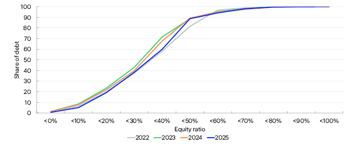
The most vulnerable CRE groups are those with both low equity ratios and weak ICRs. The share of debt in these groups increased in the period up to 2023 but has declined over the past two years (Chart 3.12). The improvement primarily reflects stronger debt-servicing capacity, while change in solvency has been less pronounced. The most exposed CRE segment remains vulnerable if earnings weaken, financing costs rise or property values fall.
Share of debt in CRE groups by interest coverage ratio and equity ratio. Percent23
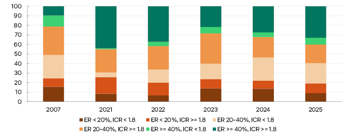
Higher long-term interest rates push up CRE yields
The rise in long-term interest rates has increased uncertainty regarding international CRE pricing and contributed to lower office segment turnover in a number of European countries. Commercial property selling prices rose at the beginning of 2025 but fell back again in 2026 Q2. Selling prices are calculated as market rental value divided by an estimated yield.24 The CRE yield has remained fairly stable in recent years even though long-term interest rates have risen. The yield fell in line with long-term interest rates in the years following the 2007–2008 financial crisis but has only partly followed the rise in rates since the pandemic (Chart 3.13).
Yield for prime real estate and ten-year swap. Percent25

An important explanation is that higher nominal interest rates have largely coincided with high inflation and a rapid rise in rents. Higher rental income has supported investor returns without a corresponding increase in the yield. In recent years, however, real interest rates have also risen. Higher real rates increase returns on alternative investments without a corresponding increase in rental income and therefore put upward pressure on the CRE yield. Market participants nevertheless point to two factors in particular that have so far helped keep the yield down:
- Strong willingness to lend and high competition among banks to extend CRE loans have put downward pressure on CRE lending margins. Credit spreads for CRE firms in the bond market have also declined, although they have recently risen somewhat. This has offset some of the rise in market interest rates. Banks continue to report strong willingness to lend but several indicate that margins are bottoming out. Higher interest rates are therefore likely to feed through to financing costs to a greater extent for leveraged CRE firms going forward.
- In recent years, the CRE transactions market has been dominated by equity investors, such as pension funds and insurance companies. These investors have played a role in pushing down the yield to a lower level than leveraged investors can compete with. So far this year, they have been less active on the buyer side, while real estate companies have accounted for a larger share of purchases in the office segment. Such developments mean that leveraged investors’ financing costs are again becoming more important for CRE pricing.
Higher office vacancy dampens rent inflation
Nominal rent inflation has long been elevated, driven by high employment and low office vacancy rates. So far this year, rents have remained unchanged and lower than projected in Financial Stability Report 2026 H1.
Slower employment growth in office-based occupations has dampened demand for office space, and office vacancy rates in Oslo have recently risen somewhat. The increase in the rates also reflects the fact that more companies are reducing their office space when entering into new leases. Some market participants highlight that such developments may be amplified by increased use of AI. However, the effects of AI on office space demand are uncertain. Increased use of AI could also boost activity and create new tasks, which could in turn increase demand.
Weaker demand for office space will likely dampen the rise in rents. At the same time, few new office buildings are expected to be completed in the coming years. This will limit the supply of office space and likely help support rents, particularly in central Oslo. Rent inflation overall is expected to be weak in 2026 but to pick up again in the coming years.
On the whole, the projections for rent inflation and the yield imply that commercial property selling prices will remain fairly flat in the coming years (Chart 3.14).26 Prices are expected to remain slightly lower over the next few years than projected in the previous Report.
Prime real estate in Oslo. Estimated selling prices. In thousands of NOK per square metre27

18 Some credit rating agencies require an ICR above 1.8 if a firm that relies on bond financing is to qualify for a high credit rating. If the ICR falls below this threshold, the bonds may be downgraded, with a marked rise in yields on new and existing bonds.
19 Period: 2016–2025 (left panel) and 2000–2027 (right panel). Projections for 2026 and 2027 from FSR 2026-2.
Interest coverage ratio is total earnings (EBITDA) as a share of total interest expenses for legal entities in real estate development.
The left panel shows total EBIDTA and total interest expenses for the same units, indexed to 2019 = 100. In the FSR 2026 H2 projections, the average interest rate is assumed to decrease by 0.06 percentage point in 2026 and increase by 0.3 percentage point in 2027, in line with the policy rate path in Monetary Policy Report 3/2026. Furthermore, operating income is assumed to increase by 4.2% in 2026 and 3.6% in 2027, while operating costs are assumed to increase by 3.3% in 2026 and 2.6% in 2027. In addition, interest-bearing debt is assumed to increase by 3.9% in 2026 and by 4.8% in 2027. In the downside scenario, the average interest rate is assumed to increase by 0.2 percentage point in 20926 and by 1.1 percentage point in 2027. Furthermore, operating income is assumed to increase by 2.3% in 2026 and decrease by 1.1% in 2027, while operating costs and interest-bearing debt develop as in the baseline scenario.
20 Consolidated financial statements provide a more comprehensive picture of the financial situation than financial statements at firm level and are therefore better suited for micro-level analyses.
21 Period: 2022–2025.
Interest coverage ratio is total earnings as a share of total interest expenses. The sample comprises CRE groups with interest-bearing debt over NOK 50m.
22 Period: 2022–2025.
Equity ratio is book equity as a share of total book assets for the individual group. Debt is interest-bearing bank and bond debt.
23 Period: 2007 and 2021–2025.
Equity ratio is book equity as a share of total book assets. Interest coverage ratio is current earnings as a share of interest expenses. Debt is interest-bearing bank and bond debt. The sample comprises CRE groups with interest-bearing debt over NOK 50m and positive earnings.
24 This yield is not the same as investors’ actual required rate of return but is a yield set by market participants based on information from real estate sales and market rents for those same properties. In general, investors’ required rate of return and therefore selling prices depend on developments in long-term interest rates and risk premiums.
25 Period: 2007 Q1-2026 Q3.
The yield is estimated as market rent divided by selling price for prime real estate in Oslo. This is a measure of direct yield and not the same as the investor’s overall required rate of return.
26 Seling prices and the projection in this Report have been calculated based on data from CBRE. The projection from Financial Stability Report 2026 H1 was calculated using data from JLL, where rent levels are different. The projections are therefore not on the same level.
27 Period: 2006 Q4–2028 Q4.
Projections from 2026 Q3 for FSR 2025 H2 and from 2026 Q2 for FSR 2025 H1.
Prime real estate is high-quality office buildings located in Vika and Aker Brygge in Oslo. Selling prices are calculated as rental prices divided by the estimated yield. The yield is based on information from real estate transactions and depends on developments in long-term interest rates and risk premiums.
3.5 Slightly higher losses on CRE exposures expected ahead
In 2026 H1, banks’ total losses on Norwegian corporate exposures remained low and in line with 2025 levels (Chart 3.15). Losses on exposures to real estate development have increased further in 2026, as expected in the previous Report. Defaults among real estate developers have also risen further over the past year and are now considerably higher than the average for the past ten years (Chart 3.16).
Recognised credit losses as a share of bank lending to the sector. Percent28
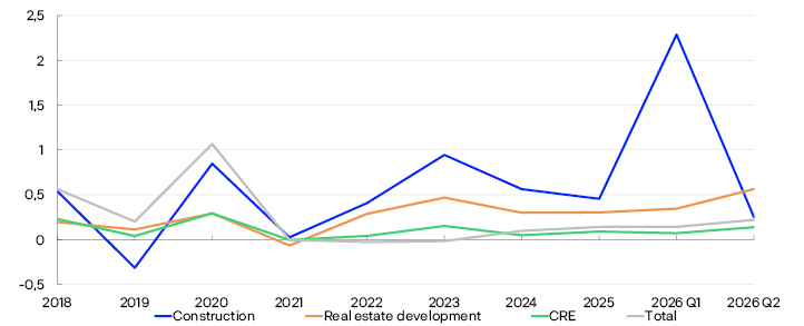
Defaults as a share of lending to the sector. Percent29

As expected, losses on CRE exposures have remained low, and the share of defaulted loans has remained low and stable. In construction, credit losses rose markedly in 2026 Q1, but the increase was mainly attributable to impairment losses on a few large exposures. Construction defaults have also increased and are at their highest level since 2018.
The share of defaults in other sectors has remained stable in recent years. Overall, the share of defaults on Norwegian corporate exposures is now lower than the average for the past ten years.
Overall credit losses on corporate exposures are expected to increase slightly in 2026 and 2027 but to remain at low levels. Even though a number of key financial figures improved last year, the current situation is eroding the liquidity buffers of many real estate developers, and continued low construction activity is expected to result in higher credit losses. In Norges Bank’s lending survey for 2026 Q3, half of banks report an increased risk of default and breach of the terms of loan covenants and a higher risk of default on loans to real estate developers. This suggests that credit risk may remain elevated. Prospects for higher financing costs and lower rental income mean that losses on CRE exposures are also expected to increase slightly but to remain low.
The outlook for credit losses is uncertain, and losses on real estate development exposures could be higher than expected. Overall, real estate developers are better positioned than a year ago, with lower debt and higher equity ratios. At the same time, margins remain tight for many firms. So far, bankruptcies have mainly involved firms with weak solvency. If construction activity remains low for a prolonged period, firms that currently appear financially sound will also draw on their buffers. If the recovery in construction activity is delayed substantially, more real estate developers could default on their loans and banks could incur larger losses on real estate development exposures than assumed.
There is also substantial uncertainty about the global economic outlook. CRE is an important channel through which external shocks can affect financial stability in Norway (Chart 1.1 in Section 1). A marked increase in long-term interest rates and risk premiums could weaken both debt servicing capacity and property values in CRE. Should employment also fall markedly and rental income prove appreciably lower than envisaged, many CRE firms could face difficulties servicing debt and refinancing loans. In a situation where many firms already have weakened profitability owing to higher financing costs, this could trigger fire sales of real estate and result in higher defaults and losses than currently envisaged.
28 Period: 2018 –2026 Q2. Annual figures for 2018–2025. Annualised figures for 2026 Q1 and Q2.
Norwegian exposures only.
29 Period: Figures for 2018 Q4–2025 and quarterly figures from 2026 Q2.
Defaults are loans that are more than 90 days past-due and other loans that banks consider to be in default. The chart shows defaults as a share of total lending to the sector. The chart shows Norwegian exposures.