1. Introduction
The purpose of this handbook is to document the expert knowledge relevant for Norges Bank’s conduct of monetary policy. Its primary focus is to elaborate on the topics and policy challenges described in Norges Bank’s monetary policy strategy statement.1 We will cite international practice and relevant literature regarding these topics and give an account of Norges Bank’s interpretations and clarifications. We will also describe the analysis system and data basis on which monetary policy decisions are based. The handbook is intended as a living product, which will be updated as the strategy and modelling system evolve.
The starting point of monetary policy is Norges Bank’s mission – its mandate – laid down by the Storting (Norwegian parliament) in law and regulation. The monetary policy framework in Norway is flexible inflation targeting. In 2001, Norges Bank was given a formal inflation target for monetary policy. In March 2018, the mandate was revised in the form of a new Regulation on Monetary Policy, specifying that the operational target of monetary policy is annual consumer price inflation of close to 2 percent over time. Furthermore, inflation targeting shall be forward-looking and flexible so that it can contribute to high and stable output and employment and to counteracting the build-up of financial imbalances.
In monetary policy, a distinction can be made between (overriding) objectives and considerations. This distinction is often related to the objectives the central bank can assume responsibility for and the objectives it cannot assume responsibility for but can contribute to. Based on this distinction, “low and stable inflation” can be considered monetary policy’s overriding objective, whereas “high and stable output and employment” and “counteracting the build-up of financial imbalances” can be regarded as considerations. Such a ranking of tasks may be appropriate for the purpose of communication, for example when articulating the responsibilities of monetary policy. However, in the practical conduct of monetary policy, the distinction is less important, because the central bank must in any case strike a balance between the different objectives and considerations in the near and medium term. For the sake of simplicity, in what follows we have used the same term – objective – for both overriding objectives and considerations.
In translating the mandate into concrete decisions, a strategy is useful. A common definition of the term “strategy” is:
A plan of action designed to achieve a long-term or overall aim.2
A monetary policy strategy describes how monetary policy should be conducted in different situations that may occur. For the strategy to be as useful in practice as possible, it should be as operational and specific as possible. The monetary policy strategy serves as a bridge from the monetary policy objectives and considerations as formulated in the mandate (Regulation on Monetary Policy) to the actual conduct of monetary policy, primarily in the form of the policy rate decision and the policy rate forecast published in the Monetary Policy Report.
|
Objectives of monetary policy |
Strategy |
Implementation |
|
Low and stable inflation with annual consumer price inflation of close to 2 percent over time High and stable output and employment Counteract the build-up of financial imbalances |
How to conduct monetary policy for best possible attainment of policy objectives? How to deal with different types of challenges (shocks, uncertainty)? |
How should the policy rate/rate path be adjusted given the strategy and economic situation? How should the decision be communicated? |
Neither the objectives nor the strategy are carved in stone but can be changed over time. However, there are differences in the degree to which they are fixed. The objectives of monetary policy are changed relatively rarely. Frequently changing the objectives could weaken confidence in monetary policy. In Norway, the monetary policy objectives have been changed twice in the past 20 years (see “The objective of monetary policy from a historical perspective”). The inflation target was formally introduced in 2001. Before that, the objective was to maintain a stable exchange rate. In the new Regulation on Monetary Policy of 2018, the inflation target was reduced from 2.5 to 2 percent. At the same time, inflation targeting was to contribute to high and stable output and employment. The word “high” was new compared with the earlier regulation, as was the phrase that monetary policy should also counteract the build-up of financial imbalances.
The strategy will be somewhat less fixed than the objectives, since the strategy should be developed as new insights are gained from research, analyses and practical experience. But substantial and frequent changes in the strategy will not be appropriate either, whether with regard to the internal decision-making process or external communication.
However, the conduct of monetary policy will, by its nature, depend on the current economic situation and the outlook. Policy rate decisions are normally made at the announced monetary policy meetings of the Monetary Policy and Financial Stability Committee (hereinafter “the Committee”). As a rule, eight such meetings are scheduled each year. In conjunction with four of these meetings, the Monetary Policy Report is published, where the policy rate forecast is an important part of the conduct of monetary policy.
The monetary policy strategy can be roughly divided into the following elements: a. specification of objectives, b. trade-off between objectives and c. response pattern.
a. Specification of objectives
For the strategy to be of practical benefit, the objectives of monetary policy must be specified so that policy performance under different policy rate scenarios can be assessed. The different objectives laid down in the mandate vary in their degree of precision. The objective of low and stable inflation is relatively precisely formulated in the mandate as “close to 2 percent over time”. It may nevertheless be appropriate to further define the phrases “close to” and “over time”. The objective of high and stable output and employment is less precise. How is “high” defined? Central banks with similar objective formulations usually relate it to “the highest level that is consistent with price stability over time”. At the same time, it is far from obvious in practice what level this is. The strategy should therefore seek to operationalise “high” so that it is possible to quantify this level. Such a quantification is naturally associated with considerable uncertainty, and the strategy should also provide some guidance on how the central bank should take uncertainty into account in monetary policy. “Counteracting the build-up of financial imbalances” is perhaps even less precise. Financial imbalances are a challenge to define and not least to estimate. Nevertheless, a strategy should seek to operationalise this consideration as far as possible, with a view to striking a balance between the objectives with some degree of consistency.
b. Trade-offs between objectives
The economic situation will normally reflect shocks of varying magnitude that have resulted in deviations from the objectives. Very often there will be a conflict, at least in the near term, between certain objectives. Part of the strategy could be to formulate some principles or criteria for what can be described as an efficient trade-off between objectives. What characterises an efficient trade-off is that performance against one of the objectives cannot be better without performance against at least one of the other objectives being poorer. With appropriate trade-offs, the performance against the various objectives will generally reflect in part the shocks that have occurred, in part the objectives’ relative importance (weight) to the decision-makers and in part the strength of the effect of monetary policy on the target variables. In addition to providing criteria for an efficient trade-off, a strategy can also be a tool for ensuring a consistent approach to weighing up the objectives over time, unless the decision-makers deliberately chose to change it.
Central banks’ weighting of objectives other than inflation is usually reflected in the time horizon for seeking to bring inflation back to the target after a deviation. A more flexible inflation targeting regime generally implies a longer horizon. The relevant horizon depends on the shocks that have occurred and whether there are conflicts between the policy required to reach the inflation target and the other monetary policy considerations.
c. Response pattern
The strategy should describe how monetary policy should be formulated depending on the shocks that might occur. Of course, it is not possible to have a detailed action plan in advance for every possible type of shock. But most shocks can be categorised as either demand shocks or supply shocks, and as either transitory shocks or persistent/permanent shocks. A strategy for how to respond to different categories of shocks will be useful for the implementation of monetary policy in practice.
Monetary policy responses to various shocks depend on how the shocks are interpreted and how they are estimated to influence future economic developments. The decision basis, which comprises different kinds of data and the modelling and analysis system, is therefore key to the monetary policy response pattern.
To assess how tight or expansionary monetary policy should be, it is necessary to have an idea of what a neutral monetary policy is, ie when monetary policy contributes to neither an increased nor decreased activity level. A key concept in this connection is the neutral real interest rate3. The neutral real interest rate changes over time, and estimates of this rate are uncertain.
The implications of uncertainty are an important part of the strategy that describes the response pattern. Uncertainty surrounds the current economic situation, the outlook and economic relationships, including the effects of monetary policy. Some types of uncertainty are not of material importance for the response pattern, while other types may imply that the policy rate should respond to shocks either more cautiously or more aggressively than otherwise. The monetary policy strategy should provide a measure of guidance on how monetary policy should relate to different types of uncertainty.
Now and then, extraordinary shocks may occur, of which the Covid pandemic and the global financial crisis (GFC) are examples. It is difficult to have a very precise strategy for such shocks since they may be very different in nature and difficult to describe in advance. Nevertheless, the strategy can contain some general guidelines for what may be a relevant response. The interaction between monetary and fiscal policy is also a relevant topic when large extraordinary shocks occur.
Section 2 contains a further specification of objectives (point a above) and trade-offs (point b), while Section 3 addresses the response pattern (point c).
Norges Bank’s Monetary Policy and Financial Stability Committee1
The Monetary Policy and Financial Stability Committee is responsible for Norges Bank’s role as the executive and advisory monetary policy authority and is responsible for the use of policy instruments to attain the monetary policy objectives. The Committee shall contribute to the promotion of financial stability by providing advice and using the policy instruments at its disposal.
The Committee consists of the governor, the two deputy governors and two external members. The external committee members are appointed by the King in Council for a term of four years. The governor chairs the Committee, and the two deputy governors are the first deputy chair and second deputy chair, respectively. The Committee became operative on 1 January 2020.
The Committee normally holds eight scheduled meetings a year, where policy rate decisions are made. Four of the meetings coincide with the publication of the Monetary Policy Report. The level of the countercyclical capital buffer is also set at these meetings.
The Committee’s meeting schedule is primarily determined by the dates of the eight monetary policy meetings. Prior to the meetings that coincide with the publication of the Monetary Policy Report, the Committee meets three times. Prior to the meetings without a report, the Committee meets once.
In 2021, the Committee held 21 meetings and two one-day seminars not directly related to the monetary policy meetings. The Committee discussed the monetary policy strategy, the strategy for the countercyclical capital buffer, the Financial Stability Report and liquidity management, among other things.
Bank staff prepare and present relevant analyses and projections that provide the basis for the Committee’s discussions and advises the Committee on policy decisions. To ensure that the discussion basis is as far as possible the same for all the Committee members, all have access to the same information and analyses provided by Bank staff.
The Committee is committed to transparent and clear external communication and seeks consensus on its assessments and decisions through in-depth discussion. The “Monetary policy assessment”, published in connection with policy rate decisions, and the “Assessment of the countercyclical capital buffer requirement”, published in connection with the buffer decisions, reflect the view of the majority. Topics of particular concern to the members in the discussions are highlighted in the assessment. Members that disagree with the assessment of the majority may dissent, and dissenting views are published together with a brief written explanation in the minutes and in the assessment published at the same time as the rate decision. All of the Committee’s decisions were unanimous in 2021. To underpin the Committee’s form as a collegial committee, the Committee chair, the governor, normally speaks on behalf of the Committee. Other Committee members may issue statements by agreement with the Committee chair.
1 The Committee’s rules of procedure contain rules for organising the work of the Monetary Policy and Financial Stability Committee and cover inter alia the Committee’s duties, the conduct of meetings and of business and the keeping of minutes (see Rules of procedure for Norges Bank’s Monetary Policy and Financial Stability Committee (norges-bank.no)).
2. Objectives and trade-offs
In most countries, the purpose of the central bank is laid down by the political authorities in a central bank act (Table 2.1). The act normally includes a primary objective to maintain monetary value or price stability. The purpose of Norges Bank’s activities is laid down by the Storting in the Central Bank Act. A new central bank act was adopted in Norway on 1 January 2020. In many countries, the purpose is more specifically defined in operational objectives, in Norway in the 2018 Regulation on Monetary Policy. In some countries, the objectives are specified in periodically reviewed agreements between the government and the central bank governor (eg Canada and Australia), or in a letter from the government to the central bank (UK and New Zealand). In others, such as the European Central Bank (ECB), the Swedish central bank (Sveriges Riksbank) and the US Federal Reserve, the central bank itself defines the operational objective. However, for these central banks too, the operational objective defined by the bank must be within the limits set by the act.
In Norway, Section 1-2 of the Central Bank Act states that the purpose of the central bank’s activities is to maintain monetary stability, promote the stability of the financial system and an efficient and secure payment system and contribute to high and stable output and employment.
The Government sets an inflation target for monetary policy through a regulation laid down pursuant to the Central Bank Act.4 Norway has had an inflation target for monetary policy since 2001. (See “The objective of monetary policy from a historical perspective” for a review of monetary policy from Norway in a historical perspective). The March 2018 Regulation on Monetary Policy reads:
Monetary policy shall maintain monetary stability by keeping inflation low and stable.
The operational target of monetary policy shall be annual consumer price inflation of close to 2 percent over time.
Inflation targeting shall be forward-looking and flexible so that it can contribute to high and stable output and employment and to counteracting the build-up of financial imbalances.
Even though the authorities have set monetary policy objectives, most central banks are free to determine the instruments they use. When we speak of central bank independence, we primarily mean instrument independence and not goal independence.
The difference between instrument independence and goal independence is not as big in practice as in principle. The objectives are often not formulated in specific detail in the monetary policy mandates. In addition, trade-offs must be made between the different objectives. This means that the central bank itself must specify, or operationalise, the objectives and make the trade-offs. The less specific the monetary policy objectives are, or the more objectives the central bank has, the more it can be said that the central bank is goal independent. An inflation target for monetary policy implies a greater degree of goal independence for the central bank than for example an exchange rate target, because inflation targeting largely entails judgement-based trade-offs between various considerations, while the policy rate under a fixed exchange rate regime is primarily given by foreign interest rates and conditions in the foreign exchange market.
In addition to the traditional monetary policy objectives – price stability and real economic stability – some central banks in recent years have given more weight to other considerations, such as climate change and income and wealth distribution. Such considerations are ordinarily not directly specified in central bank mandates, but many central bank mandates include elements supporting other government policies. The box “Climate change, the macroeconomy and monetary policy” contains a description of how central banks include climate change considerations in their monetary policy frameworks.
Central bank independence requires democratic accountability. This requirement has also been laid down in the Regulation on Monetary Policy, Section 4 of which states that Norges Bank shall regularly publish the assessments that form the basis of the implementation of monetary policy. How the central bank specifies the objectives and the trade-offs is an important part of such accountability. It is also important to the internal decision-making process and to improve the effectiveness of monetary policy. This section explores how the monetary policy objectives and considerations laid down in the mandate can be specified and how the trade-offs between them can be made in practice.
Table 2.1 Monetary policy objectives in selected countries
|
Country |
Purpose of central bank |
Operationalisation |
Monetary policy mandate |
|
Australia |
“… contribute to: - the stability of the currency of Australia; - the maintenance of full employment in Australia; and - the economic prosperity and welfare of the people of Australia.” Reserve Bank of Australia Act (1959) |
The monetary policy objective is defined in collaboration between the government and the central bank and documented in the joint agreement “Statement on the Conduct of Monetary Policy”. |
The latest agreement of September 2016 states: “They agree that an appropriate goal is to keep consumer price inflation between 2 and 3 per cent, on average over time”. It continues that this formulation provides the flexibility “to set its policy so as best to achieve its broad objectives, including financial stability”. |
|
Canada |
“… to promote the economic and financial welfare of Canada.”1 Bank of Canada Act (1934) |
The operational inflation target is defined in collaboration between the government and the central bank in a joint agreement. The inflation target is evaluated and the agreement renewed every five years. |
The latest agreement of December 2021 renewed the inflation target of 2%, measured as the mid-point of the 1–3% inflation control range. The agreement will be renewed at end-2026. |
|
Euro area |
“… to maintain price stability. Without prejudice to the objective of price stability, it shall support the general economic policies in the Union with a view to contributing to the achievement of the objectives of the Union as laid down in Article 3 of the TEU2.” |
The European Central Bank (ECB) defines the inflation target. The current strategy was adopted in July 20213. The next assessment of the strategy is expected in 2025. |
A symmetric inflation target of 2%. In July 2021 the ECB also presented a climate-related action plan. The ECB will take climate-related factors into account in its monetary policy analyses. |
|
Iceland |
“… shall promote price stability, financial stability and sound and secure financial activities.” Act on the Central Bank of Iceland (2019) |
With the approval of the government, the central bank can issue a declaration on a quantitative inflation target. |
The target is defined as a 12-month change in the consumer price index of 2½%. |
|
Japan |
“… aimed at price stability, thereby contributing to the sound development of the national economy.” Bank of Japan Act (1997) |
The BoJ specified a price stability target in January 2013. |
The inflation target is an annual rise in the CPI of 2%. |
|
New Zealand |
“…- achieving and maintaining stability in the general level of prices over the medium term; and supporting maximum sustainable employment; and … protecting and promoting the stability of New Zealand’s financial system ...”. Reserve Bank of New Zealand Act (2021) |
The finance minister issues an operational definition of the dual mandate in the form of a remit for the central bank, normally every five years. |
The latest remit came into force in March 2021. The inflation target was maintained. A new element was added requiring the central bank to assess the effect of its monetary policy decisions on government policy to support sustainable house prices. |
|
Norway |
"... to maintain monetary stability and to promote the stability of the financial system and an efficient and secure payment system. ... to promote high and stable output and employment." Central Bank Act (2019) |
The operationalisation of a stable value of money is laid down in a separate Regulation on Monetary Policy dated March 2018. |
“The operational target of monetary policy shall be annual consumer price inflation of close to 2 percent over time. Inflation targeting shall be forward-looking and flexible so that it can contribute to high and stable output and employment and to counteracting the build-up of financial imbalances.” Regulation on Monetary Policy (2018) |
|
UK |
“… – to maintain price stability, and - subject to that, support the economic policy of her Majesty’s Government, including its objectives for growth and employment.” Bank of England Act (1998) |
The price stability target and the government’s economic policy is defined in an annual remit issued by the finance minister. |
The latest remit is from March 2021. The Inflation target was reconfirmed as 2%. The mandate was also updated “to reflect the government’s economic strategy for achieving strong, sustainable and balanced growth that is also environmentally sustainable and consistent with the transition to a net zero economy”. |
|
Switzerland |
“… shall ensure price stability. In so doing, it shall take due account of economic developments.” Swiss National Bank (2003) |
The price stability target is set by the Swiss National Bank (SNB). |
The SNB lay down its monetary policy strategy in December 1999. The price stability target is annual CPI inflation of less than 2%. |
|
Sweden |
“… to maintain price stability. The Riksbank shall also promote a safe and efficient payments system.” Sveriges Riksbank Act (1988) |
The Riksbank decides how the formulations in the central bank act should be interpreted. |
The Riksbank has defined the inflation target as an annual change in the consumer price index with a fixed interest rate (CPIF) of 2%. |
|
US |
“… so as to promote effectively the goals of maximum employment, stable prices, and moderate long-term interest rates.” Federal Reserve Act (1977) |
The Federal Reserve defines its dual mandate. The first time was in 2012.4 The FOMC stated then that they assessed a long-term target of 2% inflation as consistent with the price stability objective. The Fed launched its first review of the monetary policy framework in 2019. The FOMC plans to conduct a review of the framework roughly every five years. |
After the review of the framework, two important changes were made in August 2020. The Fed now regards the inflation target of 2% as an average. Previously, the Fed reacted to deviations in employment from the Bank’s estimated maximum level of employment. The Fed will now only react to shortfalls in this level of employment. |
1 The Bank of Canada Act contains an introductory section about how the central bank was established, but the act has no objects clause.
2 Treaty on European Union
4 Statement on Longer-Run Goals and Monetary Policy Strategy. Federal Open Market Committee (FOMC). Update at the FOMC meeting in January each year. From 2019, the "statement" was reaffirmed each year in January with only minor revisions.
4 In Norway, acts are normally supplemented by regulations.
The objective of monetary policy from a historical perspective
How monetary policy has helped to maintain monetary stability has changed over time. Today, Norway has a floating exchange rate, but historically, Norwegian monetary policy has been pegged to one form or another of fixed exchange rate.1
After the fixed exchange rate regime broke down in December 1992, Norway continued to operate a more flexible exchange rate targeting regime. Even though there was not an exchange rate corridor for the krone, the orientation of monetary policy up until 1999 was primarily determined by current movements in the krone. When Svein Gjedrem became Governor in 1999, Norges Bank altered its response pattern. Instead of focusing on current movements in the krone, the key policy rate would be set so that more long-term preconditions for a stable exchange rate would be met: “Price and wage inflation which over time is on a par with euro countries is a precondition for a stable exchange rate against the euro. Moreover, monetary policy must not contribute to a downturn which undermines confidence in the krone”.2 In practice, monetary policy became oriented towards an inflation targeting regime.
An inflation target as the operational target of monetary policy was laid down in a mandate of 29 March 2001. The new regulation did not entail any material change in the monetary policy response pattern compared with the policy pursued over the two preceding years.3
Section 1 of the Regulation on Monetary Policy of 29 March
“Monetary policy shall be aimed at stability in the Norwegian krone’s national and international value, contributing to stable expectations concerning exchange rate developments. At the same time, monetary policy shall underpin fiscal policy by contributing to stable developments in output and employment.
Norges Bank is responsible for the implementation of monetary policy.
Norges Bank’s implementation of monetary policy shall, in accordance with the first paragraph, be oriented towards low and stable inflation. The operational target of monetary policy shall be annual consumer price inflation of approximately 2.5 per cent over time.
In general, the direct effects on consumer prices resulting from changes in interest rates, taxes, excise duties and extraordinary temporary disturbances shall not be taken into account.”
Although an objective of maintaining monetary stability was clearly stated in the Regulation on Monetary Policy of 2001, it had not been mentioned in the Norges Bank Act of 1985. The Regulation provided a more explicit formal and institutional anchor for monetary policy, which contributed to a greater degree of accountability. Norges Bank commented on the draft Regulation and on the consequences for the conduct of monetary policy in a letter to the Ministry of Finance on 27 March 2001.4 In the letter, Norges Bank wrote that
“[t]here has been confidence in the conduct of monetary policy. The communication of Norwegian monetary policy may nevertheless be facilitated with the Government now quantifying an inflation target, in line with international practice.”
The inflation target was set at 2.5 percent in the Regulation, while the implicit inflation target that the Bank previously followed was the level aimed for by euro area countries, ie approximately 2 percent.5 Regarding the actual numerical target, in the letter to the Ministry of Finance, Norges Bank wrote: “The inflation target of 2.5 per cent is slightly higher than similar objectives for Sweden, Canada and the euro area, but corresponds roughly to targets in the United Kingdom and Australia. The target is also approximately in line with the average inflation rate in Norway in the 1990s.”
The choice of 2.5 percent must be viewed in the context of the phasing-in of petroleum revenues, which would result in a real appreciation of the krone. The reason for choosing a slightly higher inflation target than the average rate applied by trading partners was for the real appreciation to take place gradually in the form of a widening gap in the price and cost level between Norway and its trading partners, and not in the form of a nominal appreciation of the krone.6
In the Financial Markets Report presented in spring 2016, the Ministry of Finance announced plans to assess the need to modernise the monetary policy mandate.7 The Ministry was of the opinion that the wording of the 2001 Regulation reflected the challenges that were relevant at the time.8 In the intervening period, monetary policy thinking and practice had changed. There was a desire to bring the mandate into alignment with the current conduct of monetary policy.9 10
The new mandate entered into force on 2 March 2018:
Regulation on Monetary Policy11
“Section 1 Monetary policy shall maintain monetary stability by keeping inflation low and stable.
Section 2 Norges Bank is responsible for the implementation of monetary policy.
Section 3 The operational target of monetary policy shall be annual consumer price inflation of close to 2 percent over time. Inflation targeting shall be forward-looking and flexible so that it can contribute to high and stable output and employment and to counteracting the build-up of financial imbalances.”
The most important changes comprised a downward revision of the inflation target to 2 percent from the previous 2.5 percent. The formulation contribute to high and stable output and employment replaced the formulation from the regulation from 2001 contributing to stable developments in output and employment. The word “high” is new compared with the regulation from 2001.
Also new was the inclusion of the consideration of counteracting the build-up of financial imbalances. From time to time, Norges Bank had been giving weight to this in its conduct of monetary policy within the framework of the regulation from 2001.
Stability in the krone’s value and stable expectations concerning exchange rate developments was a key element of the regulation from 2001 and helped to build a bridge from the earlier fixed exchange rate regime. However, the Ministry of Finance was of the opinion that there are good arguments to de-emphasise the krone exchange rate and exchange rate expectations as objectives per se.12 Experience has shown that the krone can be a useful shock absorber when the economy is affected by shocks. There is no reference to the krone in the new regulation.
The new Central Bank Act, which was passed by the Storting on 17 June 2019 and entered into force on 1 January 2020, confirmed the Regulation on Monetary Policy. The Act superseded the Norges Bank Act of 1985. The new Central Bank Act contains the following provision:
Section 1-2. Purpose of the central banking activities
(1) The purpose of the central banking activities is to maintain monetary stability and to promote the stability of the financial system and an efficient and secure payment system.
(2) The central bank shall contribute to high and stable output and employment.
1 See, for example, Alstadheim (2016).
2 See Gjedrem (1999).
3 See Kleivset (2012), page 40: “For the actual setting of the key policy rate, the formal policy change was less important, ‘since a monetary policy response pattern was already in place that was consistent with an inflation targeting regime’, as Gjedrem subsequently put it.”
5 The European Central Bank defined “price stability” as a year-on-year increase in the Harmonised Index of Consumer Prices (HICP) for the euro area of below 2 percent. This was subsequently clarified to “below, but close to 2 percent”.
6 See Torvik (2003) for a discussion of the argument and references to statements.
7 See Meld. St. 29 (2015–2016) Financial Markets Report 2015 (in Norwegian only).
8 See Ministry of Finance for more background on the most important changes (2018).
9 See Meld. St. 8 (2017–2018) New regulation on monetary policy (in Norwegian only).
10 See Norges Bank (2017) for a detailed account of the experience with the monetary policy framework in Norway since 2001.
11 On 1 January 2020, the Regulation on Monetary Policy from 2 March 2018 was reissued as a bestemmelse instead of a forskrift without entailing any change in the formulation. Since English does not formally distinguish between these two types of statutory instrument, this instrument is still translated as “Regulation on Monetary Policy”.
12 See Ministry of Finance (2018).
2.1 “Low and stable inflation”
2.1.1 Literature and international practice
There is a strong academic basis for the view that low and stable inflation is important for a well-functioning economy. High and unstable inflation leads to inefficient resource allocation as a result of undesirable changes in relative prices, difficulties with financial planning and inflation-induced tax distortions. Very low or negative inflation can also involve costs. Wages tend to move downwards less easily than upwards, so that some degree of inflation can make adjustments to relative wages less costly. When inflation is very low, monetary policy is also more likely to be constrained by the lower bound5 on the policy rate. There is no broad academic consensus on what defines the optimal level of inflation, but the inflation targets that are common among advanced economies are within the interval suggested in much of the literature.
Around the turn of the year 2021/22, inflation rose in most countries, owing to supply-side problems in the form of production and transport bottlenecks and to high energy prices, among other reasons. There is a discussion among economists about whether the increase in inflation is transitory or may persist. But prior to the recent rise, inflation has tended for a long time to be lower than central bank inflation targets. Many central banks have been concerned about this. The main reason for this concern is the decrease in the equilibrium real interest rate, which has reduced monetary policy space because of the policy rate’s lower bound. If inflation is too low, the challenges posed by a low equilibrium interest rate will be amplified.
A number of central banks have considered a variety of strategies to counteract the risk of inflation becoming too low and inflation expectations becoming entrenched at a below-target level. The US Federal Reserve (Fed) is the central bank that has gone furthest in its strategy, revising it in August 2020 and adopting average inflation targeting. With average inflation targeting, the central bank will, after inflation has been below target for a period, seek to subsequently bring inflation somewhat above target to “make up for” inflation that has been too low.6 By overshooting the target in this way, average inflation will be closer to the target, and this strategy may in principle better anchor inflation expectations.7
No other central bank has institutionalised an overshooting strategy such as the Fed’s, but both the European Central Bank (ECB) and the Bank of Canada (BoC) are open to the possibility of some degree of overshooting. In its Strategy Statement, the ECB writes8: “To maintain the symmetry of its inflation target, the Governing Council recognises the importance of taking into account the implications of the effective lower bound. […] This may also imply a transitory period in which inflation is moderately above target.” The BoC is a little more vague on the subject, but the following statement from their renewed monetary policy framework in December 2021 can be interpreted to mean that they are open to the possibility of some degree of overshooting as long as inflation is kept inside a tolerance band around the target9: “The Bank will also continue to leverage the flexibility of the 1–3 percent range to help address the challenges of structurally low interest rates by using a broad set of tools, including sometimes holding its policy interest rate at a low level for longer than usual.”
As for which prices, or what kind of price index, should be stabilised, theories differ somewhat. According to New Keynesian theory, which has had a strong influence on modern monetary policy thinking, monetary policy should stabilise the prices that are most rigid, ie prices that do not often change even though market conditions and costs can vary.10 In models where the exchange rate passes through fully to prices for imported goods, monetary policy should, according to New Keynesian theory, stabilise prices for domestic goods and services and not the consumer price index (CPI).11 If prices for imported goods are also rigid (gradual exchange rate pass-through), prices for imported goods should also be stabilised. In general, the prices with the highest degree of rigidity should, according to the theory, be assigned the highest weight in the price index the central bank seeks to stabilise.12
On the basis of purely theoretical considerations, the CPI may not be the optimal price index to stabilise. Nevertheless, virtually all the inflation-targeting countries target CPI inflation (Table 2.2). The main reason for this is that the CPI is an index that is well-established and understood by the general public and widely used in contracts. It is also an advantage that this index is produced by an institution outside the central bank (in Norway’s case, Statistics Norway (SSB)). Independence can underpin confidence in the inflation target.
Tabell 2.2 Inflation targeting in selected countries
|
Country |
Dual mandate |
Target |
Horizon |
|
Australia |
No |
CPI 2–3% |
Medium term |
|
Canada |
No |
CPI 2%1 |
Medium term |
|
Euro area |
No |
HCPI2 2% |
Medium term |
|
Iceland |
No |
CPI 2½% |
Average |
|
Japan |
No |
CPI 2% |
Medium to long term |
|
New Zealand |
Yes |
CPI 2%1 |
Medium term |
|
Norway |
No |
CPI 2% |
Will depend on the shocks to which the economy is exposed.3 |
|
UK |
No |
CPI 2% |
At all times, but depends on the shocks to which the economy is exposed. |
|
Switzerland |
No |
CPI, below 2% |
Medium term |
|
Sweden |
No |
CPIF4 2%1 |
Normally two years |
|
US |
Yes |
PCE5 on average 2 % over time |
Medium term |
1 Point target with a tolerance interval of ± 1 percentage point.
2 Harmonised consumer price index.
3 How quickly Norges Bank seeks to reach the target will depend on the shocks to which the economy is exposed and whether there is a conflict between the policy required to reach the inflation target and the other monetary policy considerations..
4 CPI with fixed interest rates (effects of changes in mortgage rates not included).
5 Personal Consumption Expenditure deflator.
Even though the target variable is the CPI, it may be appropriate in the operational conduct of monetary policy to focus on indicators of underlying inflation. This is because the CPI often shows short-term fluctuations that do not, or only to a limited extent, affect inflation further ahead and that the central bank therefore prefers to ‘look through’ to avoid causing unnecessary fluctuations in output and employment.
An indicator of underlying inflation can also be useful in the monetary policy trade-offs to distinguish signal from noise in inflation. Measures of underlying inflation are therefore used by many central banks as an operational guideline for monetary policy. Central banks usually use indicators that exclude the most volatile goods prices, such as prices for energy and food.
Most central banks monitor several indicators of underlying inflation. The BoC uses three measures.13 The Reserve Bank of Australia presents developments in underlying inflation using several measures in its monetary policy report.14 Some central banks have changed the indicators they give weight to without explicitly announcing the change.15
2.1.2 Norges Bank’s interpretation and assessment
The Regulation on Monetary Policy states that “[t]he operational target of monetary policy shall be annual consumer price inflation of close to 2 percent over time.” Thus, the target variable is the CPI and the target is 2 percent.16 The words “over time” and “close to” are not specifically defined in the Regulation, but reflect two conditions:
(i) Monetary policy cannot control inflation perfectly, and there is a considerable lag between changes in the policy rate and the impact on inflation.
(ii) Different types of shocks will generally occur and different objectives will have to be assessed against each other in the short term. Even if the central bank had been able to control inflation perfectly, it would not have been appropriate to keep inflation at target at all times.
As long as there is confidence that inflation will be low and stable, it is unlikely, in Norges Bank’s assessment, that fluctuations in inflation around the target will involve substantial economic costs. At the same time, the Bank will give weight in interest rate setting to avoiding large and persistent deviations from the inflation target, whether above or below the target.
Norges Bank has no specific strategy, for example overshooting, to prevent inflation from becoming too low as a result of the combination of a low equilibrium real interest rate and a lower bound on the policy rate. The Bank’s assessment is that this likely poses less of a challenge for Norway in terms of policy space than for most other countries. First, the krone has a tendency to depreciate when a global economic downturn occurs and there is substantial uncertainty. The krone depreciation pushes up inflation, thereby reducing the real interest rate for a given level of the policy rate. Second, Norway has considerable fiscal space. See Section 3.6 for a more detailed discussion of the interplay between monetary and fiscal policy.
Most central banks choose an inflation target horizon, for example two years (Table 2.2). However, the optimal horizon will generally depend on the type of shock to the economy and its size and duration. Norges Bank therefore applies a flexible horizon. The specific horizon at any one time will reflect the monetary policy trade-offs (see Section 2.4).
Norges Bank uses several indicators of underlying inflation (see “Indicators of underlying inflation”). However, the Bank’s main indicator is the CPI-ATE, which is the CPI adjusted for tax changes and excluding energy products17. It is the main indicator because energy prices in Norway, and electricity prices in particular, are highly volatile. It is also an advantage that the CPI-ATE is calculated and published by an independent institution, Statistics Norway (SSB). It has become a well-established element in Norges Bank’s monetary policy communication. However, one disadvantage of the CPI-ATE is that this indicator can include transitory price shocks that the Bank chooses to look through in monetary policy and that an indicator of underlying inflation should ideally correct for. The CPI-ATE includes volatile food prices (particularly fruit and vegetables) and volatile air travel prices, which it can often be appropriate to disregard. At the same time, changes in energy price trends can occur that the CPI-ATE does not capture, but that the Bank wishes to take into account.18 No single indicator of underlying inflation is ideal, suggesting that the Bank should look at several indicators and use judgement. For communication purposes, however, it may be appropriate to choose one main indicator.
5 Where the level of the policy rate is so low that it no longer provides stimulus to the economy.
6 In its “Statement on Longer-Run Goals and Monetary Policy Strategy”, the Fed writes: “[T]he Committee seeks to achieve inflation that averages 2 percent over time, and therefore judges that, following periods when inflation has been running persistently below 2 percent, appropriate monetary policy will likely aim to achieve inflation moderately above 2 percent for some time.” Federal Reserve Board – 2020 Statement on Longer-Run Goals and Monetary Policy Strategy
7 See Røisland (2017) for a more detailed description of average inflation.
8 https://www.ecb.europa.eu/home/search/review/html/ecb.strategyreview_monpol_strategy_statement.en.htm
9 Joint Statement of the Government of Canada and the Bank of Canada on the Renewal of the Monetary Policy Framework – Bank of Canada.
10 For international studies, see: Bils and Klenow (2004), Nakamura and Steinsson (2008). For Norwegian studies, see: Erlandsen (2014) and Wulfsberg (2016).
11 See Galì and Monacelli (2005).
12 See Aoki (2001).
13 See Bank of Canada (2016).
14 See Reserve Bank of Australia (2019).
15 See Fay and Hess (2016).
16 In the period between the introduction of the inflation target in 2001 to 2018, the target was 2.5 percent.
17 The main indicator of underlying inflation used between 2008 and 2013 was the CPIXE.
18 An indicator intended to capture this is the CPIXE, which is the CPI adjusted for tax changes and excluding temporary changes in energy prices. This indicator is constructed in the same way as the CPI-ATE but takes account of trends in energy prices instead of excluding energy prices completely, as is the case for the CPI-ATE.
Indicators of underlying inflation1
The purpose of indicators of underlying inflation is to strip out transient volatility in inflation and provide a real-time measure of trend consumer price (CPI) inflation. Some price components of the CPI tend to vary considerably from period to period. These include energy prices, which can rise sharply in one period and then fall the next. A good indicator of underlying inflation must have certain statistical properties.2 It should not deviate systematically from the CPI, be less volatile than the CPI and be able to predict future CPI inflation), it must be published at the same time as the CPI, must not be subject to revision and should be easy to understand. In addition, it is an advantage for it to be published by an independent institution.
Norges Bank uses a range of indicators of underlying inflation (Chart 1). The most important for Norges Bank’s analyses is the CPI adjusted for tax changes and excluding energy products (CPI-ATE). CPI-ATE inflation is included in the Bank’s main macroeconomic model NEMO, but other indicators are used in the Bank's inflation assessments and may influence the Bank's short-term inflation projections.
Chart 1 Indicators of underlying inflation. Twelve-month change. Percent. January 2002 – December 2021
Sources: Statistics Norway and Norges Bank
- CPI-ATE: CPI adjusted for tax changes and excluding energy products. Published by Statistics Norway.
- CPIXE: CPI adjusted for tax changes and excluding temporary changes in energy prices. Based on data from Statistics Norway but produced and published by Norges Bank.3
- CPI-XV: CPI adjusted for developments in the eight most volatile price series at group level4. Energy prices are excluded in toto. For the remaining seven5 the average change over the past six or 12 months is included. Based on data from Statistics Norway but produced by Norges Bank.6
- Trimmed mean (20%): Various sub-groups are excluded from month to month. The twelve-month change at sub-group level in the CPI is sorted in ascending order. Then the price series corresponding to 10 percent of the CPI weights at both the top and bottom of the distribution are removed. Produced by Statistics Norway and published by Norges Bank.
- Weighted median: Special case of trimmed mean. The underlying rise in prices in a given month is specified by the price change located at the fiftieth percentile ranked by the sub-groups’ CPI weights. Produced by Statistics Norway and published by Norges Bank.
- CPIM: Constructed by changing the weights in the CPI at group level. Each product group is weighted based on how well it has historically forecast total CPI one month ahead. Better forecasts result in a higher weight. Based on data from Statistics Norway but produced by Norges Bank.7
- CPI common: A measure of the common trend in the rise in prices across price series in the CPI at group level. A factor model is used to filter out price movements caused by sector-specific factors and find the trend that is common to all goods and service groups. Based on data from Statistics Norway but produced by Norges Bank.8
- Domestic CPI-ATE: A measure of the rise in prices for domestically produced goods and services. In principle, it is not an indicator of underlying inflation, but in theory and practice, it correlates more closely with domestic resource use than the total CPI. It is thus able to capture price pressures stemming from domestic factors. Based on data from Statistics Norway but produced and published by Norges Bank.
1 The box is based on Husabø (2017a).
2 See Husabø (2017a), Jonassen and Nordbø (2007), Roger (1998) and Wynne (1999).
3 See Hov (2009).
4 At group level, the CPI is divided into 39 product and service groups. At sub-group level, the CPI is divided into 93 product and service sub-groups.
5 Air fares, household textiles, fruit, coffee, tea and cocoa, vegetables, fish, newspapers, books and stationery.
6 Not published regularly.
7 See Hov (2005).
8 See Husabø (2017b).
2.2 “High and stable output and employment”
2.2.1 Literature and international practice
Setting monetary policy to achieve an inflation target does not mean that monetary policy only focuses on inflation. The mandates of inflation-targeting central banks usually include formulations indicating that real economic stability should also be considered. In the short term, conflicts can arise between stabilising inflation and stabilising the real economy, and central banks must then make a trade-off between the two.
There is a sound theoretical basis for assuming that a large share of business fluctuations involves welfare costs and should be dampened using countercyclical monetary policy.19 This is because consumers may prefer high and stable consumption, and fluctuations lead to inefficient resource allocation. The usual theoretical models assume that there is a representative household. These models do not capture all of the costs from variations in output and employment, for example that involuntary unemployment will normally involve substantial costs for an individual, and for the household. In models based on a representative household, a downturn will only entail that the household spends a little less time working. In more realistic models, which assume imperfect risk sharing and labour market frictions, for example that time and costs are associated with finding a new job, there are substantial welfare costs associated with variations in employment. Monetary policy should then stabilise employment/unemployment in addition to inflation.20
There will normally be no conflict between stabilising output and stabilising employment. Only if there are substantial fluctuations in productivity, can a conflict arise in the short term.
Both the supply and demand for labour will vary as a result of business cycle fluctuations. During downturns, when labour demand is low and job prospects are poor, labour supply will be lower than its underlying trend. For example, young people may choose to continue their education rather than seek work. Conversely, labour supply will periodically be higher than the underlying trend when labour demand is high and job prospects are favourable.
Over time, employment is limited by the underlying labour supply trend. At the same time, there will always be some unemployment in the economy. This is partly because there will always be some people who are temporarily between jobs, and because employers’ needs do not fully match the qualifications and wage expectations of those seeking work. In the literature, this is referred to as natural unemployment or equilibrium unemployment. This unemployment can change over time in response to structural changes in the labour market. The underlying labour supply trend minus equilibrium unemployment can be referred to as potential employment. This may be interpreted as the level of employment sustainable over time. If employment remains above potential, pressures normally arise that accelerate wage growth and bring inflation above target. However, there may be temporary fluctuations in labour supply for cyclical reasons. How much a given deviation in employment from potential employment affects wage growth may therefore vary.
New Keynesian literature often assumes that potential employment is lower than the socially optimal level of employment. The reasons are that firms have market power and limit output to earn higher profits by keeping price margins high, and that wage earners have market power and drive wages above a level consistent with full employment.
There is broad consensus among economists that an expansionary monetary policy can increase output and employment in the short term, but that it cannot raise these levels permanently. Attempting to keep employment permanently above potential employment will only lead to high price and wage inflation.21 To ensure price stability, the level of ambition for monetary policy should be to stabilise employment close to the highest level consistent with price stability over time.
In standard models, it is usually assumed that economic shocks are symmetric around a trend. In these models, monetary policy can only affect variations in output and employment around these trends. Stabilisation policy only affects the variance of real economic variables – not the average.
Some of the literature assumes instead that economic fluctuations are asymmetric. A pure example of asymmetric fluctuations is the “plucking” model, developed by Milton Friedman.22 In this model, negative shocks generate cyclical fluctuations, bringing output and employment below potential. Thus, potential output and employment are ceiling levels and not average levels as in standard models. If the plucking model is correct, traditional ways of estimating potential output and employment will systematically underestimate their potential levels.
Another example of asymmetry is when the occurrence of economic crises (for example financial crises) can result in downturns that are deeper and more protracted than upturns, owing to hysteresis effects in the labour market23, for example, and because high debt levels can dampen demand for a long period and reduce investment.24 If economic policy can counteract such sharp downturns, this would raise the average level of output and employment. Much of the research on this topic has focused on the role of monetary policy in counteracting crises. We will come back to this in Section 2.3.
Once a sharp downturn has occurred, monetary policy should in principle attempt to bring employment back to its pre-crisis level. A challenge with this approach is that such a policy could lead to sharply accelerating wage inflation if hysteresis effects are present in the labour market. As long as any hysteresis effects are not permanent, it may be appropriate for policymakers to accept that inflation will be above target for a period until labour market conditions normalise. More jobs could then be created, bringing back some of those who have withdrawn from the labour market.25 However, the risk of such a policy is that hysteresis effects can prove to be very prolonged or permanent. Monetary policy would then have to be tightened considerably at a later stage to bring inflation back to target.
To the extent that such asymmetries as described above exist, monetary policy can in principle not only reduce the variation in output and employment, but also, coupled with an active stabilisation policy, contribute to higher average output and employment.
Internationally, only central banks with what are referred to as dual mandates explicitly pursue the objective of high employment. The US Federal Reserve (the Fed) and the Reserve Bank of New Zealand (RBNZ) have such dual mandates, where the objectives of high employment and price stability are of equal importance. In the US, the mandate is formulated as “maximum employment26, stable prices and moderate long-term interest rates”. In 2020, the Fed affirmed that it may be necessary to target inflation of somewhat above 2 percent after a period of below-target inflation. The objective is to achieve inflation that averages 2 percent over time. At the same time, the Fed clarified that while it previously reacted to “deviations” in employment from the Fed’s estimated “employment’s maximum level”, it would now only react to “shortfalls” in employment from this level. The Fed’s strategy attempts to prevent employment falling below a maximum level. The consequence of this is that the Fed will not tighten monetary policy solely in response to what appears to be a tight labour market.
In New Zealand, a new operational monetary policy objective was added to the price stability objective for the RNBZ in 2018. The RBNZ was now to also “contribute to supporting maximum sustainable employment”27, defined as as “the highest utilisation of labour resources that can be maintained over time without generating an acceleration in inflation”.28 In 2018, maximum sustainable employment and price stability were given equal status, thereby formally instituting a dual mandate for the RBNZ.29
2.2.2 Norges Bank’s interpretation and clarification
In Norway, price stability is the primary objective of monetary policy. Even though there are similarities between the formulation “high and stable output and employment” in the Norwegian Regulation on Monetary Policy and the formulations in the dual mandates of the Fed and the RBNZ, the two objectives, price stability and high and stable output and employment, do not have equal status. In practice, however, it is not obvious that a central bank with a dual mandate would pursue a different monetary policy from a central bank with a flexible inflation target. A central bank with a flexible inflation target will also be concerned about the level of employment.
The Regulation on Monetary Policy does not itself provide guidelines on how much weight monetary policy can attach to high and stable output and employment, given that inflation expectations are firmly anchored.
In the conduct of monetary policy, the word “high” is given an operational interpretation that takes into account what monetary policy can and cannot affect. The level of ambition for monetary policy must be realistic. In line with other central banks with similar objective formulations, Norges Bank has interpreted “high” as the highest level consistent with price stability over time. If Norges Bank systematically seeks to bring employment above this level by means of an expansionary monetary policy, a period of tighter monetary policy and higher unemployment may be necessary at a later stage in order to restore price stability. The highest level of employment that is consistent with price stability over time is primarily determined by structural conditions such as the tax and social security system, wage formation and labour force composition. For example, changes in the pension system since 2011 have contributed to an increase in labour supply, while a larger proportion of elderly in the population has reduced labour supply. Monetary policy can probably have very limited impact on how high employment can become before wages and prices rise considerably, but it can contribute to stabilising employment around this level.
Norges Bank estimates an output gap, which is used as an indicator in assessing output and employment relative to the highest level that is consistent with price stability over time (see “Norges Bank’s estimates of the output gap”). When estimating the output gap, particular weight is given to labour market developments, while short-term fluctuations in labour productivity are normally disregarded. There is therefore no conflict between high and stable output and high and stable employment in the Bank’s operational interpretation of the mandate.
The economic costs of cyclical fluctuations are asymmetrical, which Norges Bank’s monetary policy response pattern seeks to take into account. Normally, an increase in employment beyond what is estimated to be the highest level consistent with price stability involves no direct costs. Only the indirect costs – wage and price inflation becoming too high – will normally prompt the Bank to seek to counteract such an increase. As long as inflation is expected to remain within a range close to 2 percent, the Bank will not normally aim to quickly close a positive output gap by tightening monetary policy unless there are signs that financial imbalances are building up. Lower employment, on the other hand, involves direct costs both in the form of losses in aggregate income and output and in the form of economic and health consequences for those unable to find employment. When the Bank estimates a negative output gap, this implies in isolation that the Bank will pursue an expansionary monetary policy to stimulate employment.
Possible hysteresis effects can also contribute to asymmetry in the costs of cyclical fluctuations. When downturns are deep and protracted, unemployment can become entrenched at a high level, with many job seekers eventually withdrawing from the labour market. Wage and price inflation can then accelerate at a lower level of employment than before the downturn. To prevent a sharp downturn from resulting in long-term or permanent falls in employment, it may be appropriate to accept that inflation will temporarily overshoot the target while labour market conditions normalise. By preventing downturns from becoming deep and protracted, monetary policy can contribute to keeping the average level of employment over time as high as possible.
19 See Galí, Gertler and Lopèz-Salido (2007). In certain models, fluctuations are efficient and should not be counteracted, but such models are based on strict and to some extent unrealistic assumptions, for example that all prices and wages are flexible.
20 See Blanchard and Galí (2010).
21 See Kydland and Prescott (1977) and Clarida, Gali and Gertler (1999).
22 See Friedman (1964, 1993). See also Dupraz, Nakamura and Steinsson (2019) for empirical support and the microfoundations of the “plucking” model.
23 Hysteresis refers to persistent unemployment that rises with every swing in the economic cycle. One explanation for this phenomenon is that in an upturn demand in the labour market is for different or a higher level of skills than the skills that became redundant in the preceding downturn.
24 See Blanchard, Cerutti and Summers (2015).
25 Such a strategy is proposed by Rudebush and Williams (2016) and Ball (2015), among others.
26 “Maximum employment” is specified as the highest employment level of employment that is sustainable over time, see Williams (2012).
27 See Monetary Policy Statement, May 2018 (Reserve Bank of New Zealand’s monetary policy report).
28 See Monetary Policy Statement, November 2018 (Reserve Bank of New Zealand’s monetary policy report).
29 See Williams (2019).
Norges Bank’s estimates of the output gap1
Norges Bank bases its assessments of the output gap on a broad set of indicators and models that are revised and expanded over time. The output gap is defined as the difference between actual and potential output. Potential output means the highest level of output and employment compatible with price stability over time. The methods used to estimate and analyse the output gap in the Bank’s analysis system are based on an assumption that cyclical fluctuations do not affect output and that the output gap will normally be close to zero in the estimates within a five-to-10-year horizon. Theories about hysteresis and about whether cyclical fluctuations can affect potential output challenge this assumption and imply that there may be other measures of potential output that take into account hysteresis effects. There are established methods for estimating this level, but this is an area that we are continuing to explore.
The output gap is not observable, and there is no widely agreed best method for estimating it. No method is without its drawbacks and all methods involve the use of judgement. As the output gap is unobservable, it is also challenging to evaluate the different methods for estimating it.
A good measure of the output gap should nevertheless satisfy certain criteria. The estimate of the output gap should have good real-time properties, ie the historical estimates of the output gap should show little change as a result of new information. Moreover, a common interpretation of potential output is output consistent with stable price and wage inflation. In periods when capacity utilisation is high and employment is growing rapidly relative to the labour force, price and wage pressures tend to increase. A good measure of the output gap should therefore provide information about future developments in inflation and wage growth. A positive output gap implies that the economy is operating above potential and that growth will eventually slow. A good estimate of the output gap should therefore provide an indication of future output growth, as well as some indication of developments in unemployment, since unemployment has historically tracked the output gap with a lag.2
Many methods can be used to measure the output gap.3 The most widely used methods are simple univariate methods (statistical filters). These methods are simple in practice and characteristically only use GDP data. The so-called Hodrick-Prescott (HP) filter is an example of a univariate method.4 There are also a number of multivariate models which, in addition to GDP data, use data on other variables. Such models have much better real-time properties and also have better real-time forecasting properties compared with simple univariate methods such as the HP filter.
To estimate the output gap, Norges Bank uses a set of multivariate models. This is because, on the whole, an average of multivariate models has featured better forecasting properties than the individual models. The models use data on both real and nominal variables. The models are based on two different multivariate methods: unobserved component (UC) models and structural VAR (SVAR) models5. In addition, Norges Bank looks at various labour market indicators when estimating the output gap.
A UC model posits that GDP can be decomposed into an output gap and potential GDP, which are both unobservable. In addition, the model specifies how the unobserved variables evolve over time. The estimation of these equations uses information about variables such as real wage growth, unemployment, business investment, inflation, credit and house prices. At Norges Bank, we estimate eight different UC models. The models differ in terms of estimation frequency, the data used, estimation period and modelling of potential growth. All of the models are estimated using Bayesian methods and are based on published articles on the output gap.6
Like the UC models, SVAR models use data from a number of variables to estimate the output gap. We estimate two SVAR models. One (SVAR 1) uses GDP growth for mainland Norway and unemployment (NAV), while the other (SVAR 2) also includes domestic inflation.
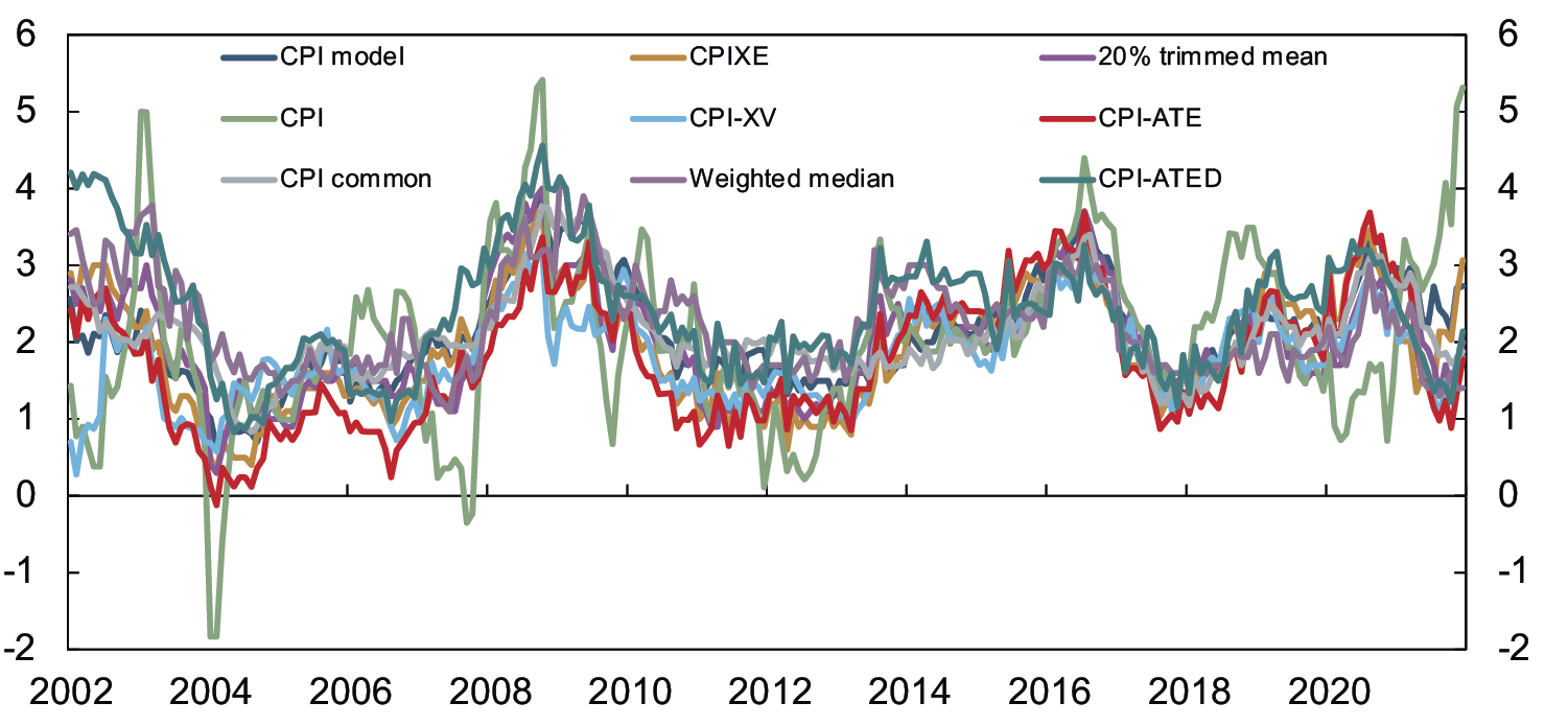
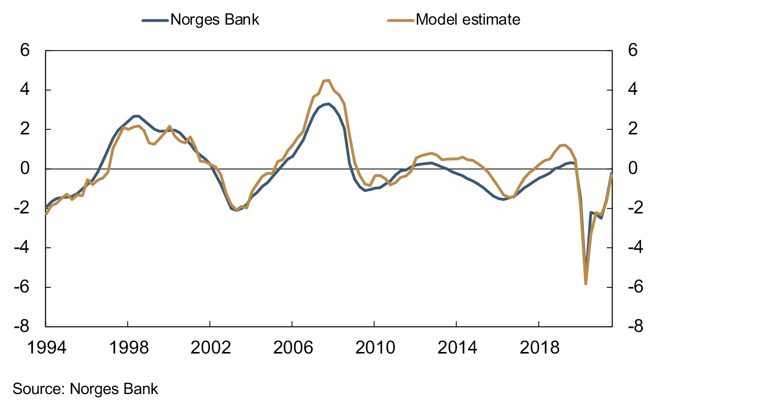
The charts below show estimates from the different models together with Norges Bank’s assessments of the output gap as presented in Monetary Policy Report 4/21. Charts 1 and 2 show estimates based on the UC models. For Chart 1, information on real wage growth, unemployment, business investment and inflation was used. For Chart 2, information on credit and house price developments was used. Chart 3 shows estimates based on the two SVAR models. Chart 4 shows an average of the models together with Norges Bank's output gap. Overall, the various models are closely in line with Norges Bank’s estimates of capacity utilisation over time.
Chart 1 Chart 1 UC models 1–6
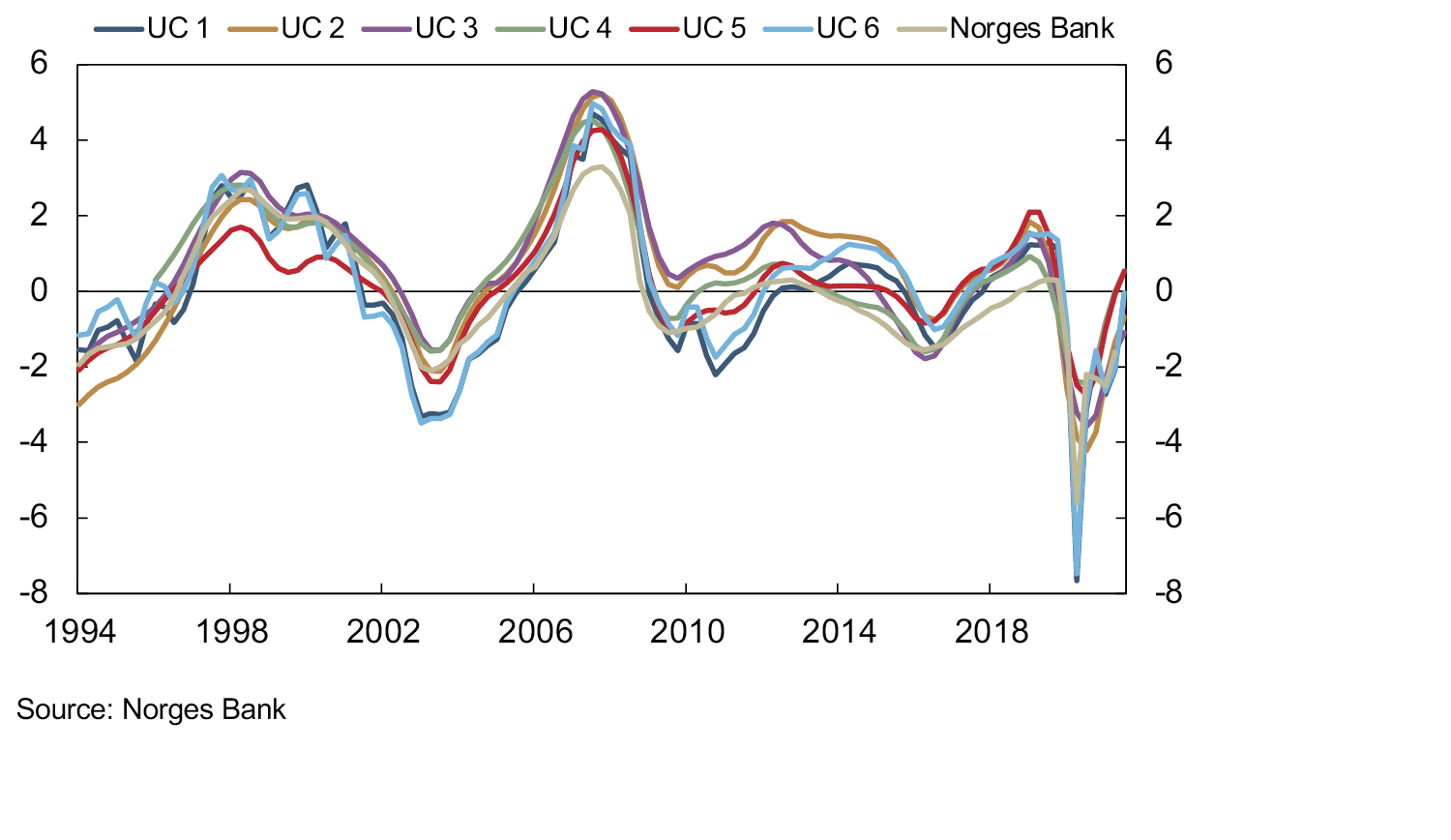
Chart 2 UC models 7–8
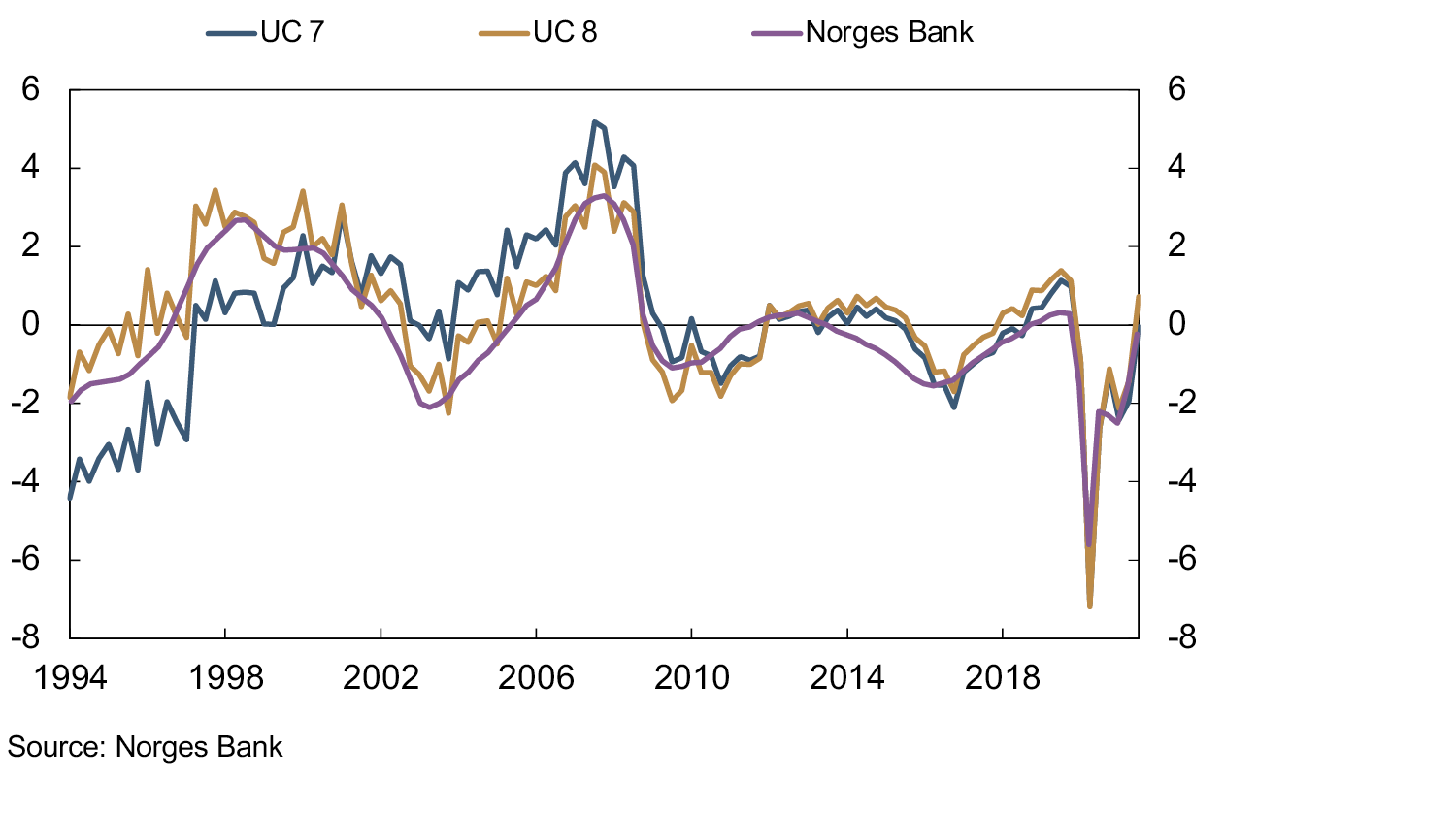
Chart 3 SVAR models
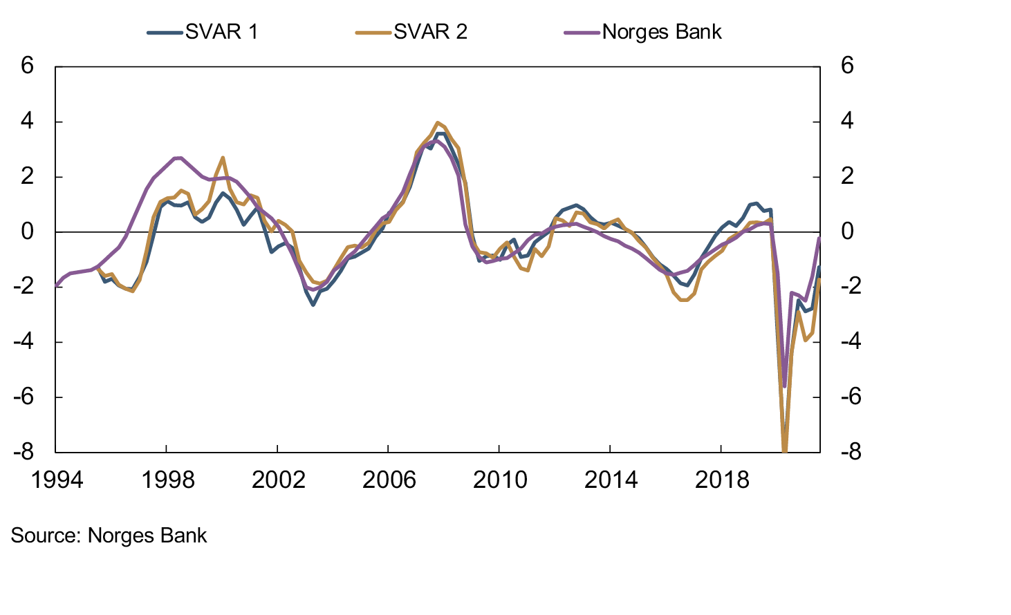
Chart 4 Model estimate
There is normally a close correlation between the gap between employment and potential employment on the one hand, and overall capacity utilisation in the economy on the other. It is not possible to measure precisely the level of potential employment. When capacity utilisation is estimated to be above a normal level, employment is usually also assessed as above potential. When capacity utilisation is estimated to be below a normal level, employment appears able to increase without the risk of accelerating price and wage inflation.
Norges Bank’s assessments of the output gap include a number of important indicators, which so far are not included in the above-mentioned models. One reason is that there is little historical data for several of these indicators. An important example of such an indicator is Norges Bank's Regional Network contacts' assessment of capacity utilisation and labour supply in the Regional Network. Norges Bank will work to include this information in the Bank's model system.
Capacity utilisation during the Covid pandemic
Assessing the output gap through the Covid pandemic has been more challenging than normal. Usually it is reasonable to assume fairly steady growth in the economy’s potential output, which reflects developments in the capital stock, working age population and productivity level in the economy. But the shutdown of the economy in 2020 was a large and unusual shock that affected both the supply and demand sides of the economy.
It was assumed that part of the fall in GDP was ascribable to a temporary decline in potential GDP. Some of the factors of production in some industries were not available owing to lockdown. For example, real capital could not be utilised by firms that had been closed.
On the other hand, there was a historic increase in unemployment. Even though much of the rise in unemployment was due to furloughs, ordinary unemployment also rose. Unemployment also increased in sectors not directly affected by lockdown. Labour market developments therefore indicated that the economic downturn triggered spare capacity in the economy and thus a negative output gap. Put another way, demand in the economy fell more than supply. The fact that the Covid crisis both reduced potential output and led to a negative output gap is well in line with assessments made by other central banks.7
Throughout the pandemic, we have also been concerned that the risk of high unemployment and an abrupt decline in employment could lead to persistently negative consequences for labour supply through what are referred to as hysteresis effects. However, in the light of the rapid recovery in employment in autumn 2021 and a continued high level of labour force participation, the projections in MPR 4/21 did not assume that long-term potential employment was being affected by the pandemic, as had been assumed previously.
1 The box is based on Hagelund, Hansen and Robstad (2018).
2 See Armstrong (2015) and Kamber et al (2017).
3 See Hjelm and Jonsson (2010) for a good overview.
4 The HP filter yields potential GDP by minimising the difference between actual and potential GDP, given a limitation on how much potential GDP growth can vary over time (see Hamilton (2017) for an extensive discussion of the HP filter).
5 Vector-autoregressive (VAR) models are stochastic models used to capture the linear relationship between time series. A structural VAR model is a VAR model on which restrictions have been imposed based on economic theory.
6 See Hagelund, Hansen and Robstad (2018) displayed.
2.3 “Counteracting the build-up of financial imbalances”
2.3.1 Literature and international practice
Financial crises are rare events, historically occurring every 15 to 20 years.30 Empirical studies show that financial crises involve higher costs than other recessions and that debt-driven upturns are associated with deeper and more persistent recessions and crises (see also Section 2.2) often referred to as “credit bites back”.31 The global financial crisis in 2008 showed that instabilities in the financial system can have very adverse macroeconomic consequences.
There is a broadly held view among central bank economists that the regulation and supervision of financial institutions, including macroprudential policy, should be the first line of defence against shocks to the financial system. Monetary policy can counter the build-up of financial imbalances by “leaning against the wind”. When there is a risk of a build-up of financial imbalances in the economy, the policy rate will be kept higher than would otherwise have been the case. The purpose is to mitigate downside risks to the economy and thus reduce the risk of financial imbalances triggering or amplifying a downturn.32 33 Since financial crises are relatively rare, the empirical basis is uncertain. However, research indicates that monetary policy can contribute to some extent to reducing the likelihood and severity of future crises.34
The cost of “leaning against the wind” is a policy rate curbing, for a period, output and inflation more than would normally be implied by the central bank’s response pattern. If the policy rate is systematically kept higher than implied by price stability considerations, this may affect average inflation over time and inflation expectations may fall.
No clear consensus has been reached, among researchers or policymakers, on whether monetary policy should “lean against the wind”. Some conclude that the benefit of “leaning”, in the form of reduced probability and severity of a crisis, is most likely lower than the costs of such a policy.35 But there are also studies that show that "leaning" may be favourable in certain situations, particularly when implemented early in a period of strong asset price inflation and credit growth.36 Among the large international institutions, the Bank of International Settlements (BIS) has long argued that central banks should “lean against the wind”37, while the International Monetary Fund (IMF) has been more sceptical.38 Different results are arrived at owing to alternative assumptions about economic relationships and the estimated effects of the policy rate on output and inflation on the one hand and financial imbalances and crisis severity on the other. The potential benefits and costs of leaning against the wind are discussed in more detail in the box “Illustration of potential costs and benefits of leaning against the wind in monetary policy”.
How financial stability considerations are taken into account differs among inflation-targeting central banks, but the main tendency is that monetary policy is rarely used to counter financial imbalances. The conclusion drawn by the Bank of Canada in connection with its regular review of its monetary policy framework is similar to the view reflected in research from the IMF.39 The Bank of Canada concluded that monetary policy should be adjusted to address financial imbalances only in exceptional circumstances and that the effective use of macroprudential tools “will reduce the incidence of significant tension between monetary policy’s objective of low and stable inflation and potential risks to financial stability”. In its most recent review of monetary policy in December 2021, the Bank’s view was very similar to the view expressed in 2016. The Bank wrote the following: “The Bank will continue to assess financial system vulnerabilities, recognising that a low interest rate environment can be more prone to the development of financial imbalances. A variety of other policy instruments, such as macroprudential tools, are better suited than monetary policy to address these vulnerabilities. But because monetary policy can exacerbate financial vulnerabilities, the Bank will continue to be mindful of the risk that such vulnerabilities can lead to worse economic outcomes down the road.”40
The US Federal Reserve (the Fed) has expressed scepticism about using the policy rate to counter financial imbalances other than as an option if other alternatives should prove not to function.41 In August 2020, the FOMC published a new “Statement on Longer-Run Goals and Monetary Policy”. In the statement, the consideration of financial stability was noted explicitly: “Moreover, sustainably achieving maximum employment and price stability depends on a stable financial system. Therefore, the Committee’s policy decisions reflect its longer-run goals, its medium-term outlook, and its assessments of the balance of risks, including risks to the financial system that could impede the attainment of the Committee’s goals”.
In its new monetary policy strategy, the European Central Bank (ECB) appears open to greater flexibility in responding to the downside risks arising from financial imbalances42. The ECB writes that: “The monetary and financial analysis also provides for a more systematic evaluation of the longer-term build-up of financial vulnerabilities and imbalances and their possible implications for the tail risks to output and inflation.”43
According to the new Reserve Bank of New Zealand Act44, in addition to its existing monetary policy objectives of “achieving and maintaining stability in the general level of prices” and “supporting maximum sustainable employment”, the Reserve Bank of New Zealand (RBNZ) also has a “financial stability objective of protecting and promoting the stability of New Zealand’s financial system”. In addition to monetary policy, the RBNZ is also responsible for the supervision of financial institutions. In February 2021, the Ministry of Finance decided that the RBNZ shall explicitly explain how monetary policy decisions support the government’s housing policy of more sustainable house prices.45 At the same time the RBNZ shall take house prices into account when making decisions related to the financial stability mandate.
In the period between mid-2010 and a few years ago, Sveriges Riksbank’s monetary policy “leaned against the wind”.46 The Riksbank was worried about the rapid rise in household debt and house prices over some time. To curb the rise in house prices and debt, the policy rate was set slightly higher than would otherwise have been the case. When inflation did not rise as expected and inflation expectations fell after a period, the Riksbank abandoned “leaning against the wind” to avoid undermining confidence in the inflation target. The policy rate was set at negative levels for a period and alternative instruments were subsequently introduced, such as the purchase of government bonds. See Section 3.5 for a further discussion on alternative instruments.
It has become more common in recent years to quantify risk associated with financial imbalances by using a “Growth-at-Risk” framework.47 The framework is empirical and can be used to link measures of financial imbalances to forecasts of downside risk in the economy somewhat further ahead. The IMF actively uses this framework when monitoring financial stability.48 One of the findings in this literature is that expansionary financial conditions (eg high house price inflation and credit growth) may lead to reduced downside risk for the economy in the short term (around one year), but higher downside risk in the medium-term (around three years). In a situation with weak developments in output, employment and inflation, a balance must therefore be struck between the benefits of an expansionary monetary policy stance in the short term and the risk that vulnerabilities build up and make targets more difficult to achieve further out. Conversely, a contractionary monetary policy stance can lead to greater near-term downside risk, but greater future benefit as household and corporate deleveraging can lead to a reduced risk of downturns. If households and non-financial firms are highly vulnerable at the outset, it may require particularly demanding trade-offs.49
It is difficult in practice to decide whether central banks “lean against the wind” to some extent as monetary policy should in any case respond to changes in financial variables because these variables have an impact on activity levels. Perhaps the difference between central banks that “lean” (at times) and central banks that do not appear to “lean” is less in practice than indicated by the literature and debate.
2.3.2 Norges Bank’s interpretation and clarification
The Regulation on Monetary Policy states that inflation targeting shall counteract the build-up of financial imbalances, which increases the risk of a sharp downturn further out. The consideration of mitigating financial imbalances therefore derives from the consideration of high and stable output and employment over time.
Monetary policy cannot take primary responsibility for mitigating the build-up of financial imbalances. As in international practice, in Norges Bank’s assessment, the regulation and supervision of financial institutions are the most important tools for cushioning shocks to the financial system.
A persistently low interest rate level can sow the seeds of increased risk-taking, soaring property prices and rapid debt accumulation. High debt makes households and firms more vulnerable to income shortfalls, augmenting the risk of a severe downturn in the future. If there are signs that financial imbalances are building up, the consideration of longer-term stability may warrant maintaining a somewhat higher policy rate than the consideration of high and stable output and employment in the short term may suggest.
Setting a higher policy rate to mitigate the build-up of financial imbalances may involve costs in the form of lower near-term demand. In the Bank’s monetary policy assessments, reducing the risk of a severe downturn in the long term is weighed against maintaining high and stable output and employment in the near term. In many situations, the degree of conflict between the two considerations will be minimal. In an upturn, for example, house prices and credit will also tend to rise sharply. A tighter monetary policy stance will then contribute to both greater near-term stability and a lower risk of a severe downturn further out. In a situation where the risk of a severe downturn is acute, both the need to stabilise the real economy and maintain financial stability could suggest a rapid reduction of the policy rate as this could counteract a sharp decline in asset prices, which could have triggered or amplified a downturn.
In some situations, short-term and longer-term stability may be more at odds. In a downturn, the policy rate will normally be lowered to cushion the contraction. Even though a lower level of economic activity also dampens house price inflation and debt growth, a lower policy rate will in isolation, stimulate the housing market. Such stimulus will often be desirable and contribute to dampening the decline in economic activity, but in some cases house price inflation and credit growth can rise to such a high level that they conflict with the aim of long-term stability. This would then provide grounds for lowering the policy rate somewhat less or starting to normalise the policy rate slightly earlier than suggested by the need to support activity in the short term.
For monetary policy to counteract the build-up of financial imbalances and weigh this consideration against other objectives, it is an advantage if the view on what “imbalances” are is as precise as possible. Defining and estimating “financial imbalances” is difficult. Norges Bank’s interpretation of financial balances has been linked to the risk of sharp economic downturns further out. Periods of sharp property price inflation and credit growth and an underpricing of risk are associated with higher risk of severe downturns. Risk is often defined as the product of probability and impact. Financial crises are rare events. Imbalances, probability and impact are difficult to quantify and model owing to few historical observations. In addition, the relationship between financial imbalances and risk is nonlinear and complex. Norges Bank’s assessment of financial imbalances will largely be based on a number of indicators and an overall judgement.50
30 See Taylor (2015).
31 See Jordà, Schularick and Taylor (2013).
32 Financial stability considerations are primarily linked to the risk of sharp economic downturns, but there may also be other reasons for stabilising financial variables. In recent years, economic literature has shown that large movements in asset prices, such as house prices, can result in random distributional effects and create uncertainty about the future scope for consumption.
33 The benefit is particularly high if economic agents underestimate the risk of a crisis and if crisis dynamics are amplified by financial imbalances. See Gerdrup, Hansen, Krogh and Maih (2016).
34 See BIS (2016).
35 See Svensson (2016), Ajello et al (2016) and Pescatori and Lasèen (2016).
36 See Ajello et al (2016) and Guorio et al. (2016).
37 See Borio (2014) and Juselius et al (2016). See also Borio (2016) and Filardo and Rungcharoenkitkul (2016).
38 IMF (2015). The report concludes that the response pattern of monetary policy should probably not be adjusted to take account of financial stability because the policy rate is too blunt an instrument for financial stability purposes, and because there most often will not in any case be a conflict between the objectives of stable output and inflation and the objective of financial stability. The report also emphasises that it is not always easy in real time to determine the strength of an economic upturn.
39 See letter of 21 September 2016 to the Minister of Finance from the Governor of the Bank of Canada in connection with the renewal of the inflation target. https://www.bankofcanada.ca/wp-content/uploads/2016/10/Letter-Minister-Finance.pdf
41 See Yellen (2014), Brainard (2017) and Quarles (2019).
44 The bill was passed by Parliament on 10 August 2021.
45 See press release of 25 February 2021, https://www.rbnz.govt.nz/news/2021/02/rbnz-supports-focus-on-housing
46 See Ingves (2019).
47 See eg Adrian, Boyarchenko and Giannone (2019) and Aikman, Bridges, Hoke, O’Neill and Raja (2019). For an empirical application of Norwegian data see Arbatli et al (2020) and Albertsen (2020).
48 See IMF (2017).
49 See Liang and Adrian (2019). https://www.brookings.edu/blog/up-front/2019/04/11/how-growth-at-risk-can-help-central-bankers-gauge-financial-stability-risks/
50 For an overview of the various indicators used to monitor financial stability, see Arbatli and Johansen (2017).
Illustration of potential costs and benefits of leaning against the wind in monetary policy
To illustrate potential costs and benefits of leaning against the wind, we begin with a study by Kockerols, Mimir and Kravik (2021).1 The study is based on a variant of Norges Bank’s macroeconomic model, NEMO, in which crises can occur. The model contains a banking sector that provides loans to households and firms and a housing sector. For households, a dwelling is both a consumer durable and collateral. This gives rise to two mechanisms. First, increased demand for housing will lead to higher house prices, and second, higher house prices will make it easier for households to debt-finance consumption and investment.
In normal times, banks and the housing market will rarely be the source of substantial macroeconomic shocks in the model, but in this variant of the model, high credit growth will both increase the probability of a financial crisis occurring and lead to greater falls in output if a crisis were to occur.2 Moreover, a key assumption is that households and firms systematically underestimate the risk that a financial crisis can occur.
In the model, the central bank makes a trade-off between stabilising the deviation of output from potential output and the deviation of inflation from the inflation target. The box “Modelling objectives and trade-offs: Loss functions” describes how the central bank’s objectives and trade-offs can be presented mathematically with the aid of loss functions. The trade-off between stable output and stable inflation can be illustrated by the following loss function:

where Lt is the expected “loss” in a given period t, πt is inflation, π* is the inflation target, yt is the output gap and β is a discounting factor. Et expresses expectations based on information available at time t and may be interpreted as the central bank’s forecast. As (1) shows, the expected loss is higher the further away from the targets actual inflation and output are expected to be. The deviations are squared, ie the central bank’s losses increase with wide deviations from the targets in either direction.
Alternatively, the loss function can be expressed as follows3:

The first two terms in this expression mean that the expected loss is greater the wider the inflation and output gaps are. The last two terms mean that the expected loss is greater the more uncertainty there is in the projections. In linear models, it is sufficient to assess the point forecasts for inflation and the output gap to determine whether there is an appropriate balance between output and inflation. However, a model that incorporates the possibility of a crisis will be non-linear. In such a model, an important channel for monetary policy will also be to influence the variance in the variables. A reduction in the build-up of financial imbalances will then mitigate the downside risk to the economy and thus reduce expected variation in the output gap and inflation further out.
The cost associated with leaning, as it can be estimated within this framework, is illustrated by a temporary 1 percentage point increase in the interest rate over four quarters. The interest rate increase is assumed to reflect the fact that for a period the central bank is seeking to mitigate the build-up of financial imbalances to a greater extent than what is consistent with the central bank’s typical response pattern. As shown in Chart 1, such a rate increase results in a decline in output and inflation. This contributes to higher expected losses as assessed by the central bank (see loss function (2) above).
The benefits of the interest rate increase are reaped further out in time owing to lower credit growth and hence a reduced probability of a financial crisis (Chart 2). The expected fall in output during a crisis, given that it materialises, is also reduced. This is because households and firms are less vulnerable to a downturn when there is less build-up of debt prior to a crisis. This latter benefit is greater further out in time, since it takes time for financial imbalances to recede. A lower downside risk to the economy reduces the expected variation in the output and inflation gaps and thus contributes to a lower expected loss expressed by the last two terms in function (2).
Total costs and benefits will depend on the economic situation prior to the interest rate increase, which follows from the quadratic loss function. Furthermore, the probability of a crisis is not linear. This means that the probability of a crisis changes less when imbalances are low at the outset than when they are high. Chart 3 shows an estimate of cumulative net benefits per quarter (t) when the economy is in balance to start with, ie that the output gap is closed, inflation is at target and there are no financial imbalances. The purple bars show cumulative costs owing to weaker output and inflation developments. These costs arise quickly and are not reversed. Besides the output gap and inflation being under the targets on account of the interest rate increase, the costs increase to an additional extent when a crisis amplifies the poor performance in achieving objectives. Cumulative gains owing to a lower expected crisis probability (orange bars) and less serious downturns (blue bars) increase somewhat after some time but are not large enough to compensate for the increased costs. This means a net loss (Lt> 0).
Chart 4 shows the result of an exercise similar to the one in Chart 3, but where financial imbalances are increasing. Technically speaking, financial imbalances are increasing as a result of a temporary increase in housing demand and a subsequent large increase in house prices and credit. In this case, the costs of leaning against the wind will be somewhat less than in Chart 3, since the increase in demand also has an expansionary effect on the economy (purple bars). At the same time, the benefit of leaning is greater since monetary policy contributes to reducing financial imbalances (orange bars). As stated above, the probability of a crisis is not linear. This means that a given fall in financial imbalances leads to a greater reduction in the probability of a crisis when it is high at the outset. After some years, the higher interest rate overall will contribute to a net benefit (Lt < 0).
The estimations of gains and losses are highly uncertain. This is partly because periods of financial instability occur relatively infrequently and because structural conditions in the economy and the financial system imply divergent risks of financial instability across countries. If the interest rate has a pronounced effect on the build-up of financial imbalances, the benefit of leaning is greater as it reduces the risk of a sharp downturn further ahead in time. If the interest rate has a pronounced effect on output and inflation, the short-term costs of allowing the interest rate to respond to financial variables are greater.
Chart 1 Effect on inflation and the output gap of a four-quarter monetary policy shock. Inflation. Percentage points. Output gap. Percent
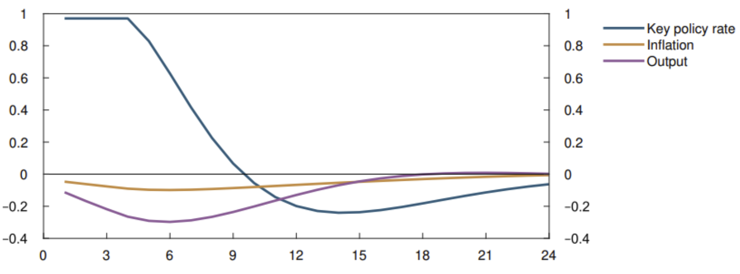
Source: Kockerols, T., Y. Mimir and E. Kravik (2021)
Chart 2 Probability of a crisis from a four-quarter monetary policy shock. Quarterly probability of a crisis arising. Percent
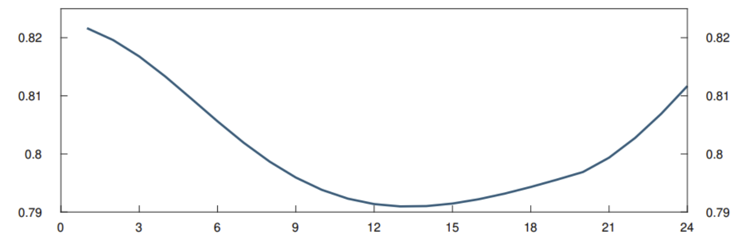
Source: Kockerols, T., Y. Mimir and E. Kravik (2021)
Chart 3 Effect on expected cumulative costs and benefits1) from a monetary policy shock that lasts for four quarters when the economy is in balance at the outset
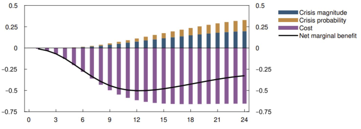
1 Costs (-) and benefits (+) are defined as the cumulative sum of the output and inflation gaps when both elements are squared.
Source: Kockerols, T., Y. Mimir and E. Kravik (2021)
Chart 4 Effect on expected cumulative costs and benefits1) from a monetary policy shock that lasts for four quarters when financial imbalances increase markedly at the same time
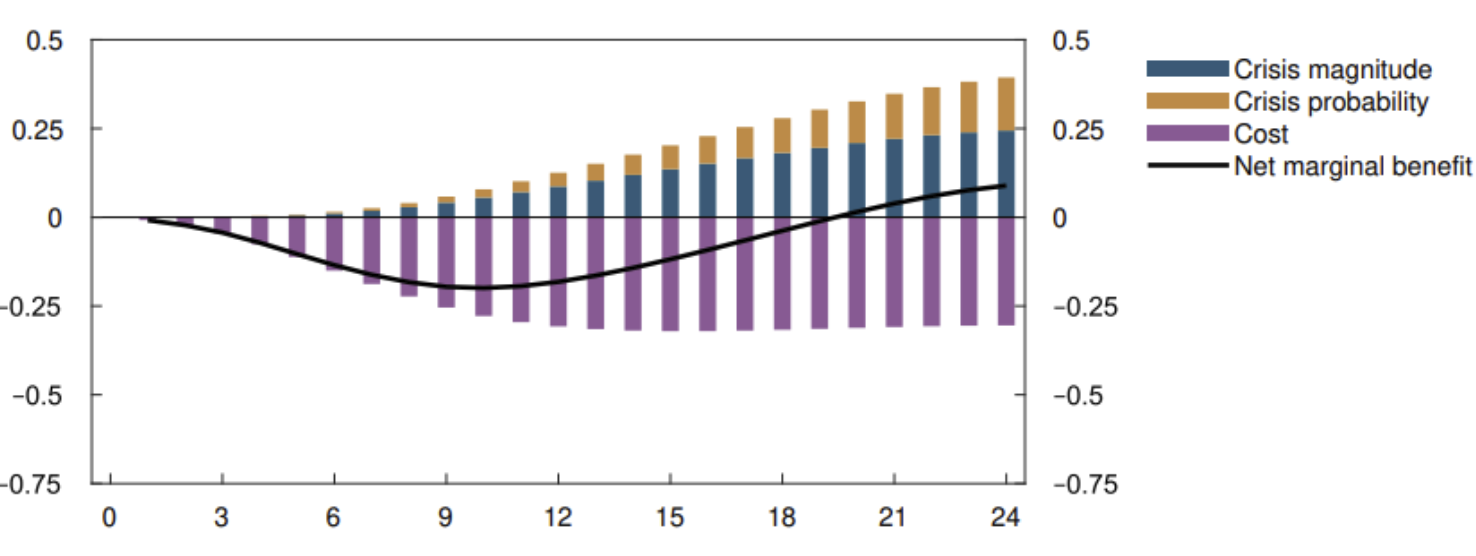
1 Costs (-) and benefits (+) are defined as the cumulative sum of the output and inflation gaps when both elements are squared.
Source: Kockerols, T., Y. Mimir and E. Kravik (2021)
1 Kockerols, T., Y. Mimir and E. Kravik (2021). Similar exercises with a more stylised model have been described in Gerdrup, K., F. Hansen, T. Krogh and J. Maih (2017).
2 See also Jorda, O., M. Schularick, and A. M. Taylor (2013) for information based on longer historical data series.
3 Here the definition of conditional variance is used: vart(xt+k) = Et(xt+k – Etxt+k)2
2.4 Trade-offs between monetary policy objectives
Trade-offs between monetary policy objectives are largely based on judgement. Nevertheless, there may be grounds for some guidance for such trade-offs in monetary policy strategy. First, such guidance could improve the internal decision-making process and contribute towards more consistent trade-offs over time. Second, it would lead to a better public understanding of how the central bank makes trade-offs between various objectives and considerations. This may strengthen confidence in monetary policy and improve accountability.
As described above, three objectives are specified in Norges Bank’s monetary policy mandate51:
1. consumer price inflation close to 2 percent over time,
2. high and stable output and employment, and
3. counteracting the build-up of financial imbalances.
There will often be a short-term conflict between some of these objectives. Striking a balance between the various objectives is an important part of monetary policy.
2.4.1 Literature and international practice
Good trade-offs have two requisite characteristics. First, better performance in achieving one objective should not entail poorer performance in achieving the others. That is, trade-offs must be efficient. Second, the degree to which the various objectives are achieved must reflect (i) the central bank’s assessment of the importance of the different objectives, (ii) the effect of monetary policy on the objectives and (iii) the type of shock that has occurred (including the size and duration of the shocks).
An efficient trade-off often implies that the inflation gap (the difference between actual inflation and the 2 percent inflation target) and the output gap (the difference between actual and potential growth) have different signs.52 For example, if both gaps are negative, a more expansionary monetary policy may bring inflation closer to target and output closer to its potential level. If there are more than two objectives, for example if the consideration of counteracting the build-up of financial imbalances is also taken into account, there could be situations where it is efficient for the inflation gap and the output gap to have the same sign. See “An indicator for the weight given by Norges Bank to financial imbalances and other considerations” for an analysis of deviations from the simple rule that the inflation gap and the output gap should have opposite signs, primarily owing to the consideration of counteracting financial imbalances. In many models with forward-looking rational expectations, it would be optimal for gaps to have the same sign for several periods after the occurrence of a shock, also when there are only two objectives.53
Monetary policy operates with a lag, with the largest impact of the policy rate on inflation and GDP normally occurring between one and two years after the policy rate has been changed. Therefore, in practice, inflation targeting means inflation forecast targeting. The Swedish economist and former Deputy Governor of the Riksbank Lars Svensson has had considerable influence on the research on inflation targeting and has shown in many of his papers how optimal flexible inflation targeting can be implemented.54 Svensson’s main principle is that the central bank should determine an interest rate path with corresponding inflation and output forecasts so that the expected loss, measured using a loss function with an inflation gap and output gap/unemployment gap, is reduced as much as possible. However, Svensson’s approach to optimal flexible inflation targeting has been criticised by many, partly because it does not give sufficient weight to uncertainty and because the model may be misspecified.55
In practice, the degree of flexibility in inflation targeting has been linked to the time horizon for achieving the inflation target. The more weight the central bank places on the real economy (a higher lambda; see “Illustration of potential costs and benefits of leaning against the wind in monetary policy” for a more detailed explanation) and the slower the monetary policy transmission mechanism, the longer the optimal time horizon for achieving the objective.56 The optimal horizon also depends on the type and duration of shocks. A supply-side shock, which leads to a greater conflict between price stability and stability of the real economy, implies a longer optimal horizon than a demand shock.
Over time, inflation-targeting countries have tended to extend the target horizon. This change does not seem to be a result of a change of opinion regarding how quickly monetary policy has an impact but reflects the authorities’ experience and increased understanding of the shocks that can occur. Inflation targeting has become more flexible.57 The greater flexibility may also reflect the greater importance in the early phase of inflation targeting of building confidence in the inflation target, which could imply a less flexible inflation targeting regime.
Today, most inflation-targeting countries operate with a medium-term time horizon (Table 2.2). A medium-term horizon for achieving the inflation target generally implies that some weight is also given to other targets. A medium-term time horizon has the advantage of being able to anchor inflation expectations and permit short-term deviations from the target when the economy is exposed to shocks.58 Extending the horizon does not appear in general to have weakened confidence in central banks.59 Indeed, this change may have been possible because the credibility of the inflation targeting regime has increased over time.
In the recent period, a number of central banks, including the Bank of England, the ECB and the Riksbank, have signalled their intention also to take climate-related considerations into account in the conduct of monetary policy (see “Climate change, the macroeconomy and monetary policy”. The more considerations monetary policy must take account of, the more difficult the trade-offs will be. There is a vigorous debate among academics and practitioners around the world about whether it desirable and/or possible for central banks to take climate-related considerations into account in the conduct of monetary policy.
2.4.2 Norges Bank’s interpretation and clarification
The policy rate path is intended to provide a reasonable trade-off between the various monetary policy objectives. What is a reasonable trade-off is primarily based on judgement, and the monetary policy mandate does not provide clear guidance on how to strike a balance between objectives.
In principle, an assessment of the importance of the various objectives is reflected in their weights in the loss function. Loss functions are discussed in further detail in the box “Modelling objectives and trade-offs: Loss functions”. In Norges Bank’s main model NEMO, the policy rate assumptions and other variables are derived based on the minimisation of a loss function.
As described in Section 2.3, it is difficult to operationalise financial imbalances in terms of a concrete variable or indicator. In the box “An indicator for the weight given by Norges Bank to financial imbalances and other considerations”, we estimate, based on a single indicator, the extent to which the Bank has made judgement-based trade-offs involving considerations other than (the forecast for) inflation and the output gap. The consideration of counteracting the build-up of financial imbalances in particular has led the Bank to decide to deviate from a reasonable trade-off between the forecasts for the inflation gap and the output gap. But the consideration of uncertainty as to the effects of the policy rate has probably also played a part. (See Section 3.4 for further discussion about uncertainty.)
As described above, it has been common practice among inflation-targeting central banks to let the trade-off between the inflation target and other targets and considerations be represented in the choice of horizon for achieving the inflation target. In the first few years after the introduction of inflation targeting in Norway, Norges Bank had a two-year horizon. This was then common practice for inflation-targeting central banks. The horizon gradually became more flexible, and perhaps the Bank’s horizon was more flexible than the horizon of other inflation-targeting central banks. This has been expressed by inflation projections that have often not returned to target within the projection horizon in the Bank’s monetary policy reports, which is about three years.
The Bank does not currently specify any particular horizon. How quickly the Bank seeks to return inflation to target will depend on the shocks that have occurred and whether there are conflicts between the policy stance needed to reach the target and other monetary policy considerations. To specify how the horizon depends on the degree of conflict between the objectives, the Bank writes in its strategy that it will normally seek to set the policy rate to bring up inflation faster if economic activity is low than if activity is high. Correspondingly, in a context of above-target inflation, the Bank will aim to bring down inflation faster when activity in the real economy is high than when activity is low.
51 As stated in Section 2.1, the term objective is used for both objective and consideration.
52 See Røisland and Sveen (2018).
53 This is because by promising to set the policy rate so that the inflation gap and the output gap have the same sign in the future, a benefit can be achieved today. For example, if a negative inflation shock occurs, the effect on inflation today would be less if the central bank commits itself to setting a policy rate that leads to high inflation and thus a positive output gap in the future because forward-looking firms take this into account when determining current inflation. See Clarida, Galì and Gertler (1999).
54 See Svensson (2010).
55 See Orphanides (2007).
56 See Smets (2000).
57 See Paulin (2006).
58 See Hammond (2012).
59 See Paulin (2006).
Modelling objectives and trade-offs: Loss functions
It is common in the literature to present monetary policy objectives with the aid of a “loss function”. The policy rate paths generated by NEMO are based on this kind of loss function. The term “optimal policy” is often used for the monetary policy derived by minimising a loss function in a given model.
The loss function is intended to reflect decision-makers’ preferences in the trade-off between objectives. Like all models, a loss function is simplification of reality, where assumptions are made inter alia about the function’s form. A possible “translation” of the Regulation on Monetary Policy to a loss function is as follows:

where πt is inflation in period t, π* is the inflation target, yt is output and y* is the highest level of output compatible with price stability. y can also be an employment target. λ is the weight decisions-makers place on stability in output/employment relative to the weight on stable inflation. Lt measures the loss in each period, but monetary policy is to be forward-looking and minimise an expected discounted loss:
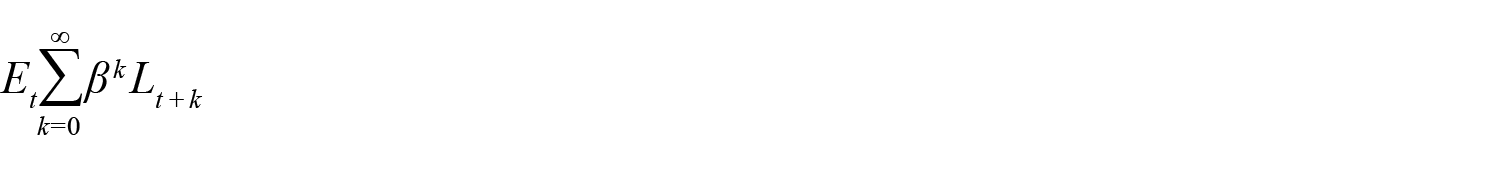
where β is the discounting factor. In this loss function, deviations from the targets are squared. This is a common assumption, for which there are several reasons. First, such an assumption is often necessary to solve for an optimal policy in the model. Second, quadratic loss functions treat deviations from the targets symmetrically. For example, below-target inflation is just as “costly” as corresponding above-target inflation. Third, quadratic loss functions entail that narrow deviations from the target mean little, eg that inflation is 2.1 and not 2.0 percent, while wider deviations have considerable bearing. Given the uncertainty about the “optimal” inflation rate for an economy and challenges in measuring inflation precisely, such a modelling of the costs of deviations from the target may seem reasonable. The same considerations apply to deviations from the level of output/employment compatible with price stability.
It is not necessarily the case that the central bank’s attitude to deviations from the targets is always symmetrical. For example, Norges Bank considers deviations in employment from the highest level compatible with price stability as asymmetrical; there are appreciable costs associated with negative deviations from yt* while there are no costs associated with positive deviations, only indirect costs in the form of wage and price inflation (see Section 2.2.2). To take account of this, one can either specify an asymmetrical loss function, which makes estimation of the optimal policy more complicated, or one can make judgement-based deviations from the optimal policy with the aid of “monetary policy shocks”, so that the policy rate path better represents policymakers’ true preferences.
The Regulation on Monetary Policy also states that monetary policy shall contribute to counteracting the build-up of financial imbalances. It is not obvious how this consideration can be modelled in the loss function. It may be argued that the consideration of financial stability is not a separate objective but is derived from the consideration of high and stable output and employment over time. Financial imbalances can increase the risk of sharp economic downturns, ie a sharp decline in yt further ahead. If the relationship between financial imbalances and the risk of sharp downturns is well represented in the model, minimising the loss function in (1) will result in a policy that provides an optimal monetary policy response to financial imbalances. In that case, there is no need for an extra expression in the loss function to represent financial imbalances.
However, in practice it may be appropriate to capture the consideration of counteracting financial imbalances with a separate expression in the loss function. There are two reasons for this: First, modelling the relationship between the stability of the real economy and financial imbalances poses a considerable challenge. Second, modelling such relationships fairly realistically will make the model cumbersome. This suggests a simple model, where the risk of sharp downturns is not modelled explicitly, but which is limited to the relationship between the interest rate and financial variables such as debt growth, house prices and other financial variables associated with increased risk of future downturns. The consideration of financial stability can then be modelled by adding an expression for financial imbalances to the loss function as follows:

here, ft is a relevant financial variable, or aggregate of several financial variables, and ft* is its equilibrium value. Even though this may be a simpler way of modelling the consideration of counteracting financial imbalances than seeking to build the relationship between financial variables and the risk of severe downturns into the model itself, finding a relevant indicator and assigning a reasonable weight in the loss function is not unproblematic. Empirical analyses can provide some support, but this approach primarily involves seeking to model the exercise of judgement in a systematic, but simplified way.
Like the output gap/employment gap, there are reasons for the financial gap to be included asymmetrically and not squared in the loss function. Financial stability concerns are generally greater if house price inflation and debt growth are higher than a normal level than if they are lower.
A risk associated with asymmetric targets is that they can lead to monetary policy biases. For example, a tendency to set a higher policy rate than otherwise if the financial gap is positive but not a correspondingly lower rate if the gap is negative could in isolation lead to average inflation that is too low. There may, however, be other asymmetries that can result in biases that are opposite in sign, such as the above-mentioned asymmetry in the output gap. The net effect of various biases on average inflation is in principle very difficult to estimate.
The loss function in the Bank’s main model, NEMO, used as the basis for deriving the policy rate path, is:

Currently, the Bank does not operate with an aggregate indicator, ft, for financial imbalances, but uses various indicators and judgement-based assessments when performing assessments of financial imbalances. Instead, the Bank uses an expression for the deviation in the interest rate from the normal rate, (it – i*)2, to address some of this consideration. Intuitively, there is a greater risk of financial instability when the interest rate deviates substantially from its normal level.1 In addition, the weight of the output gap is higher than otherwise, because there is a correlation between high aggregate demand and high house price inflation and credit growth.
In the Bank’s operational loss function, an expression is also included for changes in the interest rate, (it – it–1)2. This expression is called “interest rate smoothing” and is commonly included in loss functions of this kind, even though interest rate smoothing is not an objective in itself. The primary motivation for interest rate smoothing is to obtain more realistic policy rate paths in line with decision-makers’ preferences. Optimal policy without this expression tends to result in bigger changes in the interest rate than what is observed in practice. Central banks normally take a slightly gradual approach to interest rate setting, for reasons that are not necessarily captured by the model. Interest rate smoothing can also be motivated by its ability to have a favourable effect on agents’ expectations.2
However, given the characteristics of this kind of model, the weights in the loss function will not necessarily reflect decision-makers’ assessments of the importance of the various targets. The specification of the loss function must be viewed in the context of how the entire model is specified, where the primary consideration is to model the Bank’s historical response pattern. A change in the specification or quantification of the model will generally result in a somewhat different response pattern. Changes in the model must therefore often “counteract” changes in the loss function for the response pattern emerging from the model to be consistent with the Bank’s historical response pattern.
Judgement should be used in all use of models for policy purposes. The policy rate paths derived from NEMO and the loss function above will always be assessed and adjusted on the basis of judgement and other information. Because both the model and the loss function are simplifications, the weights in the loss function are not necessarily constant over time but may depend on factors not captured by the modelling system. In some cases, it may be correct to give weight to considerations other than those included in the loss function. Nevertheless, optimal policy will be a useful starting point for policy discussions and an aid for checking whether the response pattern is consistent over time.
1 See Evjen and Kloster (2012).
2 Goodfriend (1991) ) shows that interest rate smoothing better enables the central bank to influence long-term interest rates. Woodford (2003) shows that interest rate smoothing provides a “gain from commitment” by making monetary policy history-dependent, which contributes to more stable inflation.
An indicator for the weight given by Norges Bank to financial imbalances and other considerations
Norges Bank’s monetary policy mandate specifies three objectives: 1) inflation of close to 2 percent over time, 2) high and stable output and employment, and 3) counteracting the build-up of financial imbalances. Norges Bank’s performance with regard to 1) can be measured directly by the inflation gap, ie the gap between inflation and the inflation target, while the Bank’s performance with regard to 2) can be measured by the Bank’s estimates of the output gap. To what extent Norges Bank gives weight to counteracting the build-up of financial imbalances is difficult to measure directly as there is no good indicator of financial imbalances. It is nevertheless possible to estimate indirectly how far the Bank has “leant against the wind”, ie set a different policy rate than that implied in isolation by objectives 1) and 2). We have developed an indicator called LOC (Leaning and Other Considerations) that reflects the extent to which the Bank appears to have given weight to considerations other than inflation and output/employment in a narrow sense. The consideration of counteracting the build-up of financial imbalances is the most obvious, but not the only, consideration, and we will come back to this.
The LOC indicator is based on a simple loss function with an inflation gap (deviation in inflation from the inflation target) and an output gap1 (see “Modelling objectives and trade-offs: Loss functions”):

Financial imbalances are not explicitly included in this loss function. However, minimising the loss function may incorporate the consideration of counteracting financial imbalances by taking into account the relationship between financial imbalances and the risk of sharp downturns further out. Therefore, with a “correct” model, this loss function may be sufficient to satisfy the monetary policy mandate.
Substantial work has been done, both internationally and at the Bank2 to model the relationship between financial imbalances and the risk of a sudden shift in demand further out with the aid of financial indicators. However, modelling these relationships poses a considerable challenge. In addition, any realistic modelling of these relationships will make the model cumbersome. The consideration of financial stability is therefore primarily addressed by judgement-based trade-offs “outside the model”.
Besides the consideration of financial stability, there may be other considerations that are not sufficiently captured by the modelling system and that also must be addressed by judgement-based trade-offs “outside the model”. Such factors may be uncertainty about the effect of interest rate changes, including in situations with unusually low interest rates, or other undesirable side effects than those directly associated with financial stability.
In a simple model, the first order condition for an optimal policy will be for the weighted sum of the inflation and output gaps to be zero.3 Therefore, an optimality criterion is for the two gaps to have different signs. If the weighted sum of the gaps is different from zero, it implies that the cental bank has taken other considerations into account than those captured by the loss function (1) and the simple model:

We have chosen to use forecasts five-12 quarters ahead as the basis for the indicator in our benchmark for taking account of the lag in monetary policy. The shorter the horizon, the better the indicator will reflect the current situation, since it takes time for shocks to die out. For longer horizons, we have a more solid basis for stabilising the output gap and bringing inflation closer to the target.
We have also chosen as a starting point to have the gaps be included with the same coefficient (τ=1). Given that an interest rate change appears to have twice the effect on output as on inflation at around the two-year horizon, the same coefficient for the two gaps in the indicators implies a value for λ in the loss function (1) of around 0.5. We have also calculated the indicator for λ =0.2, which results in a coefficient (τ) for the output gap in the LOC indicator of 0.4.
Chart 1. LOC indicator and alternative with lower weighting of the output gap and the policy rate
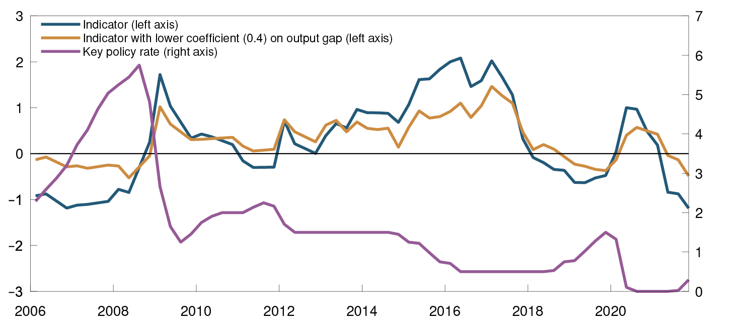
Source: Norges Bank
Chart 1 shows the LOC indicator from 2005.4 As the chart shows, the indicator has been positive for most of that time, which indicates that the Bank has often taken other considerations into account that imply a higher policy rate. This has often been with the aim of counteracting the build-up of financial imbalances. However, in some periods, the indicator has been negative, ie we have taken account of considerations that imply a lower policy rate than warranted by the outlook for inflation and the output gap in isolation. It is difficult to envisage that the Bank has wished to stimulate house price inflation and credit growth by themselves. Periods when the LOC indicator has been negative can likely be explained by other considerations. First, uncertainty about the effect of the policy rate implies a more cautious approach to policy rate setting (see Section 3.4.2), which in some situations may mean that both the inflation gap and output gap forecasts may be positive. Second, periods when a negative LOC indicator largely reflects a positive output gap may be the result of the Bank’s asymmetric view of the output gap, where a positive gap does not involve, or involves to a lesser extent, a “loss”, in contrast to a negative output gap (see Sections 2.2.1 and 2.2.2).
Over time, the LOC indicator clearly covaries with the policy rate. Concerns about financial imbalances have typically arisen when the policy rate has been set at low levels and has been low for a period, and then used as an argument against further rate reductions or for a faster rate hike. In such periods, there may be considerable uncertainty about whether further stimulus, in the form of a lower policy rate or flatter rate path, will have a normal effect on output, employment and inflation. But in those situations, the room for further stimulus has also been more limited.
Chart 2. LOC indicator decomposed by the average forecast for the output and inflation gaps one to three years ahead
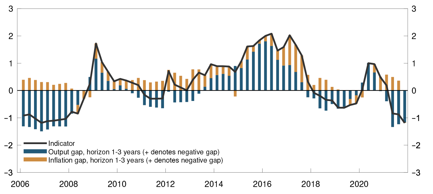
Source: Norges Bank
Chart 2 shows developments in the LOC indicator decomposed by the contributions from the output and inflation gaps five-12 quarters ahead. Generally positive values for the inflation gap contribution throughout the period reflect the fact that the medium-term inflation forecasts have typically been below the target. The output gap makes a positive contribution to the LOC indicator when the medium-term forecasts are generally negative. This was particularly the case in the wake of the oil price fall in 2014. During the pandemic, the output gap fell sharply. With the gradual reopening of society and economy recovery, the output gap forecasts increased to positive levels through 2021. The medium-term inflation forecast has often been lower than the inflation target and contributed in isolation to an increase in the LOC indicator.
1 It is also customary to include a term for “interest rate smoothing”, which punishes changes in the interest rate. The primary motivation for interest rate smoothing is to obtain more realistic policy rate paths in line with decision-makers’ preferences.
2 For modelling of the relationship between financial imbalances and monetary policy “leaning”, see Gerdrup, K. R., F. Hansen, T. Krogh, and J. Maih (2017). A similar exercise based on Norwegian data (NEMO) is documented in Kockerols, T., Y. Mimir and E. Kravik (2021). See Arbatli-Saxegaard, E., K. Gerdrup and R. Johansen (2020) for further information on the relationship between financial imbalances and downside risk for the economy.
3 See Røisland and Sveen, “Monetary policy under inflation targeting” Norges Bank Occasional Papers 53/2018.
4 There is no point in basing the indicator on inflation and output gap forecasts prior to 2005 Q3, since they are based on an exogenous policy rate path, which generally does not represent the Bank’s best trade-offs between the two considerations.
Climate change, the macroeconomy and monetary policy
Climate change and mitigation measures affect the macroeconomy and financial markets. For that reason, although the political authorities have the responsibility for mitigating climate change and have the most appropriate instruments at their disposal, climate-related changes have a bearing on central banks’ mission to promote economic stability. Central banks have therefore built expertise and increased the allocation of resources to understand the potential implications of climate-related changes for monetary policy, the outlook for financial stability and central bank balance sheets. International collaboration to address climate change has also been intensified, particularly through the climate network of central banks and financial supervisors, the Network for Greening the Financial System (NGFS).1
Macroeconomic effects of climate-related changes
Both the effects of climate change, such as more extreme weather, a higher global temperature and rising sea levels, and the transition to a low-carbon economy affect the economy in many ways.2 The effects can take the form of transitory shocks or more long-term, structural changes and can be transmitted through several channels:
- Inflation, the real economy and employment can be affected, for example, by extreme weather events that can damage crops, factories and infrastructure3 and by climate mitigation measures such as higher carbon prices.4
- The functioning of the economy can be affected, for instance because the transition to a low-carbon economy can change the structure of the economy or because the impact of climate-related changes can vary across different groups and sectors.5 From a monetary policy perspective, the impact on productivity in the transition period is also a key issue. Another important consideration is how uncertainty about future climate-related changes – climate risk – is affecting investment decisions and asset prices today.6
- Climate change can also have an impact on the monetary policy trade-offs. Extreme weather events, for example, can pull inflation and output in different directions and can – if the impact persists – make the monetary policy trade-offs more demanding.7 (cf. discussion in Section 3.4).
- The neutral real interest rate, which is the rate that creates a balance between aggregate demand and output capacity, can be affected because climate-related changes can have an impact on potential output in an economy.8 Uncertainty about future climate-related changes can also affect the neutral real interest rate.9
Climate-related work and international monetary policy
Many central banks are now working to integrate climate change considerations into the analytical framework for monetary policy. The European Central Bank (ECB), which published a comprehensive action plan to address climate change in July 2021, is committed to strengthening its analytical capacity in macroeconomic modelling, statistics and monetary policy to take climate change considerations into account.10 The Bank of Canada has also announced that it has begun to develop new models and data sources to better understand climate-related effects on the Canadian economy.11 It will assess, among other issues, the implications of more frequent disruptions from severe weather events and the transition to a low-carbon economy for potential output, the labour market and inflation. Other central banks such as those of New Zealand, Japan, the UK, Sweden and Denmark have signalled that they will increase their attention on how climate-related changes are affecting the country’s economy.12
Whether central banks should contribute to mitigating climate change, for example by using monetary policy instruments, is the subject of international debate.13 Over the past year, several central banks, including Sweden’s central bank, the Riksbank14, the Bank of England15, the ECB16 and the Bank of Japan17, have announced that they will include, or are considering including, climate change considerations in their use of some monetary policy instruments. More specifically, the Riksbank, the Bank of England and the ECB have signalled that they are taking or may take sustainability into account in their corporate bond purchase programmes (“green QE”), while the Bank of Japan is offering a sustainability-related lending facility for financial institutions.
Central banks’ motivation for including climate change considerations in their use of monetary policy instruments varies somewhat. The Bank of Japan seeks to stabilise the macroeconomy in the long term by supporting the private sector’s green transition through the new lending facility. The ECB gives weight to the potential effect of climate change on price stability and will therefore, within its mandate, contribute to addressing climate change. The ECB also explains its decision to incorporate climate considerations into its policy framework in terms of support for the EU’s climate policies. The ECB has, like many other central banks,18 a mandate to support government economic policies, as long as this is not at the expense of the central bank’s primary objective. The Bank of England, whose monetary policy mandate was updated to include climate considerations in March 202119, has launched “green QE” to support an orderly transition to a net zero economy.20 The Riksbank is also seeking to take account of sustainability in its asset purchases to enable it to contribute to climate change mitigation and include climate risk considerations.
Climate-related work and monetary policy at Norges Bank
In Norway, the primary monetary policy instrument is the policy rate (see Section 3.1). The policy rate is not an appropriate instrument to address climate change, but measures to reduce carbon emissions may affect the structure of the Norwegian economy and thereby the monetary policy stance. In addition, the increased global frequency of extreme weather events, caused by climate change, may affect the Norwegian economy and make the monetary policy trade-offs more demanding. In periods of structural changes and considerable uncertainty, such as related to climate change, it can be even more important for monetary policy to contribute to price stability and stability in the real economy.
Norges Bank works to enhance our understanding of how climate change and the transition to a low-carbon economy affects macroeconomic developments and monetary policy.21 So far, Norges Bank’s work has included conducting two surveys among the enterprises in the Bank’s Regional Network about how climate-related changes are affecting enterprises’ operations,22 analysing how climate change is affecting mainland investment23 and contributing to a research report on climate risk and commodity currencies.24
In the period ahead, Norges Bank will continue to build knowledge about how climate change and the transition to a low-carbon economy are affecting the Norwegian economy and incorporate this knowledge into the Bank’s monetary policy analyses. The Bank will also continue to collaborate with other stakeholders, through for example participation in international fora such as the NGFS.
1 At 15 December 2021, the NGFS, established in December 2017, comprised 105 members and 16 observers. Norges Bank became a member of the NGFS in December 2018. See NGFS for more information.
2 See for example Batten, Sowerbutts and Tanaka (2020), NGFS (2020a) and the box on climate change in Monetary Policy Report 1-2021 (norges-bank.no).
3 See Parker (2018) for the impact of natural disasters on inflation in different countries.
4 See Konradt and Weder di Mauro (2021) and Metcalf and Stock (2020) for the empirical effects of higher carbon prices on inflation and GDP and employment, respectively.
5 See for example Reserve Bank of New Zealand (2021).
6 Empirical studies show that climate risk can among other things affect share prices, bank lending and exchange rates, see for example Bolton and Kacperczyk (2021), Kacperczyk and Peydró (2021) and Kapfhammer, Larsen and Thorsrud (2020).
7 See for example Matsen (2019).
8 See Bylund and Jonsson (2020) and ECB (2021).
9 See Dietrich, Müller and Schönle (2021).
10 See Climate change and the ECB and ECB (2021) for more information.
12 See Our approach to climate change – Reserve Bank of New Zealand, The Bank of Japan’s Strategy on Climate Change, Climate change | Bank of England, The Riksbank’s Climate Report and Climate change and the role of central banks – Nationalbanken.
13 See Dikau and Volz (2021)
14 See Andersen and Stenstrøm (2021). The Riksbank also takes sustainability considerations into account in its management of the foreign exchange reserves, see The Riksbank’s Climate Report.
16 See ECB presents action plan to include climate change considerations in its monetary policy strategy
18 According to an NGFS survey among 107 central banks, about half have a mandate containing a formulation that monetary policy shall support the government’s economic policies (see NGFS (2020b)). Usually, this goal is formulated as a secondary goal for monetary policy.
21 See the box in Monetary Policy Report 1-2021 (norges-bank.no).
22 The survey results were published in Brekke and Erlandsen (2020) and Brekke, Eger and Erlandsen (2021).
23 See the box in mpr_221.pdf (norges-bank.no).
24 Kapfhammer, Larsen and Thorsrud (2020).
Literature
Adrian, T., N. Boyarchenko and D. Giannone (2019) “Vulnerable Growth”. The American Economic Review 109(4), April, pp 1263–89.
Aikman, D., J. Bridges, S. Hacioglu Hoke, C. O’Neill and A. Raja (2019) “Credit, capital and crises: a GDP-at-Risk approach”. Staff Working Paper No. 824. Bank of England.
Ajello, A, T. Laubach, J.D. Lopez-Salido and T. Nakata (2016) “Financial Stability and Optimal Interest-Rate Policy”. Finance and Economics Discussion Series 2016-067, Board of Governors of the Federal Reserve System.
Alstadheim, R. (2016) “Exchange rate regimes in Norway 1816–2016”. Staff Memo 15/2016. Norges Bank.
Aoki, K. (2001) “Optimal monetary policy responses to relative-price changes”. Journal of Monetary Economics, Vol. 48(1), August, pp 55–80.
Arbati, E.C and R. M. Johansen (2017) “A Heatmap for Monitoring Systemic Risk in Norway”. Staff Memo 10/2017. Norges Bank.
Arbati-Saxegaard, E.C., K. R. Gerdrup and R. M. Johansen (2020) “Financial imbalances and medium-term growth-at-risk in Norway”. Staff Memo 5/2020. Norges Bank.
Armstrong, J. (2015) “The Reserve Bank of New Zealand’s output gap indicator suite and its real-time properties”. Analytical Notes 8, Reserve Bank of New Zealand.
Ball, L. (2015) “Monetary Policy for a High-Pressure Economy”. Center on Budget and Policy Priorities. 30 March.
Bank of Canada (2016) Renewal of the inflation-control target. Bank of Canada, October.
Batten, S., R. Sowerbutts and M. Tanaka (2020) “Climate Change: Macroeconomic Impact and Implications for Monetary Policy”. In: Walker T., Gramlich D., Bitar M. and Fardnia P. Eds. Ecological, Societal, and Technological Risks and the Financial Sector. Palgrave Studies in Sustainable Business in Association with Future Earth. Palgrave Macmillan, Cham.
Bils, M. and P. J Klenow (2004) “Some Evidence on the Importance of Sticky Prices”. Journal of Political Economy, Vol. 112 (5), pp 947–987.
BIS (2016) “86th Annual Report”. Bank for International Settlements, 26 June.
Blanchard, O. and J. Galí (2010) “Labor Markets and Monetary Policy: A New Keynesian Model with Unemployment”. American Economic Journal: Macroeconomics, 2(2), April, pp 1–30.
Blanchard, O., E. Cerutti and L. Summers (2015) “Inflation and Activity – Two Explorations and their Monetary Policy Implications”. NBER Working Paper No. 21726.
Bolton, P. and M. Kacperczyk (2021) “Do investors care about carbon risk?” Journal of Financial Economics, Vol. 142 (2), November, pp 517–549.
Borio, C. (2014) “Monetary policy and financial stability: what role in prevention and recovery?”. BIS Working Papers No 440.
Borio, C. (2016) Towards a financial stability-oriented monetary policy framework? Speech at “Central banking in times of change”, the Central Bank of the Republic of Austria, September.
Brainard, L. (2017) Rethinking monetary policy in a new normal. Address to the conference Rethinking Macroeconomic Policy. Peterson Institute for International Economics, Washington D.C.
Brekke, H. and S. K. Erlandsen (2019) “Klimatilpasninger i næringslivet” [Climate-related adjustments in the business sector], blogpost published on Bankplassen blogg 19 May 2020 (in Norwegian only).
Brekke, H., F. Eger and S. K. Erlandsen (2021) “Norske bedrifter ser forretningsmuligheter i klimaomstillingen” [Norwegian businesses see business opportunities in the climate transition], blogpost published on Bankplassen blogg 2 June 2021 (in Norwegian only).
Bylund. E and M. Jonsson (2020) “How does climate change affect the long-term real interest rate?”, Economic Commentaries No. 11, Sveriges Riksbank.
Clarida, R., J. Gali and M. Gertler (1999) “The Science of Monetary Policy: A New Keynesian Perspective”. Journal of Economic Literature, 37 (4), December, pp 1661–1707.
Dietrich, A., G. Müller and R. Schonle (2021) “The Expectations Channel of Climate Change: Implications for Monetary Policy”. Discussion Paper 15866, Centre for Economic Policy Research (CEPR).
Dikau, S. and U. Volz (2021) “Central bank mandates, sustainability objectives and the promotion of green finance”. Ecological Economics, Vol. 184, June.
Dupraz, S., E. Nakamura and J. Steinsson (2019) “A Plucking Model of Business Cycles”, NBER Working Paper, No. 26351, National Bureau of Economic Research.
Erlandsen, S. (2014) “Sticky prices and inflation expectations in Norway”. Staff Memo 15/2014. Norges Bank.
ESB (2021) “Climate change and monetary policy in the euro area”. European Central Bank Occasional Paper Series No 271, September.
Evjen S. and T.B. Kloster (2012) “Norges Bank’s new monetary policy loss function – further discussion”. Staff Memo 11/2012. Norges Bank.
Fay, R. and K. Hess (2016) “Monetary Policy Frameworks: Recent international Developments”. Bank of Canada Review, Spring 2016.
Filardo, A.J. and P. Rungcharoenkitkul (2016) “A quantitative case for leaning against the wind”. BIS Working Papers No 594.
Friedman, M. (1964) “The Monetary Studies of the National Bureau”, The National Bureau Enters Its 45th Year, National Bureau of Economic Research, pp 7–25.
Friedman, M. (1993) “The ‘Plucking Model’ of Business Fluctuations Revisited”, Economic Inquiry, Vol. 31, No 2, pp 171–177.
Galí, J. and T. Monacelli (2005) “Monetary Policy and Exchange Rate Volatility in a Small Open Economy”. The Review of Economic Studies, Volume 72, Issue 3, July, pp 707–734.
Galí, J., M. Gertler and J.D. López-Salido (2007) “Markups, Gaps, and the Welfare Costs of Business Fluctuations”. The Review of Economics and Statistics, MIT Press, Vol. 89(1), pp 44–59.
Gerdrup, K.R., F. Hansen, T. Krogh and J. Maih (2016) “Leaning Against the Wind When Credit Bites Back”. International Journal of Central Banking, Vol. 13 No. 3, September, pp 287–320.
Gjedrem, S. (1999) Challenges to economic policy. Address to the Norwegian Association of Economists in Gausdal, Norway, 28 January (in Norwegian only).
Goodfriend, M. (1991) Interest rates and the conduct of monetary policy. Carnegie-Rochester Conference Series on Public Policy, Vol. 32, pp 7–30.
Guorio, F., A.K. Kashyap and J. Sim (2016) “The Trade-offs in Leaning against the Wind”. IMF Annual Research Conference, 29 October.
Hagelund, K., F. Hansen and Ø. Robstad (2018) “Modellberegninger av produksjonsgapet” [Model estimates of the output gap]. Staff Memo 4/2018. Norges Bank (in Norwegian only).
Hamilton, J. (2017) “Why You Should Never Use the Hodrick-Prescott Filter”. Working paper (see Hamilton’s home page: http://econweb.ucsd.edu/~jhamilton/).
Hammond, G. (2012) “State of the art of inflation targeting – 2012”. Handbook No. 29, Centre for Central Bank Studies. Bank of England.
Hjelm, G. and K. Jönsson (2010) “In Search of a Method for Measuring the Output Gap of the Swedish Economy”, Working paper No. 115, National Institute of Economic Research.
Hov, M. (2009) “Teknisk beregning av KPIXE” [Technical calculation of the CPIXE]. Staff Memo 3/2009. Norges Bank (in Norwegian only).
Hov, M. (2010) “CPIM: a model-based indicator of underlying inflation”. Economic Commentaries 6/2010. Norges Bank.
Husabø, E. (2017a) “Formulation of the inflation target. In: Røisland, Ø. Ed. “Review of flexible inflation targeting (ReFIT). End of project report.” Occasional Papers 51/2017. Norges Bank.
Husabø, E. (2017b) “Indicators of underlying inflation in Norway”. Staff Memo 13/2017. Norges Bank.
IMF (2015) “Monetary Policy and Financial Stability”. Staff Report, September.
IMF (2017) “Global Financial Stability Report”, October.
Ingves, S. (2019) Swedish monetary policy experiences after the global financial crisis – what lessons are there for other countries?, Address to the Money Macro and Finance Research Group, 15 October.
Jonassen, M. and E. Nordbø (2007) “Indikatorer for underliggende inflasjon i Norge” [Indicators of underlying inflation in Norway]. Penger og Kreditt 3/2006, pp 166–175. Norges Bank (in Norwegian only).
Jordà, O., M. Schularick and A.M. Taylor (2013) “When credit bites back”. Journal of Money, Credit and Banking, 45 (2), December, pp 3–28.
Juselius, M., C. Borio, P. Disyatat and M. Drehmann (2016) “Monetary policy, the financial cycle and ultralow interest rates”. BIS Working Papers No. 569.
Kacperczyk, M. and J. L. Peydró (2021) “Carbon Emissions and the Bank-Lending Channel”. CEPR Discussion Paper DP16778, December.
Kamber, G., J. Morley and B. Wong (2017) “Intuitive and reliable estimates of the output gap from a Beveridge-Nelson filter”. Discussion paper DP2017/1. Reserve Bank of New Zealand.
Kapfhammer, F., V. H. Larsen and L. A. Thorsrud (2020) “Climate risk and commodity currencies”. Working Paper 18/2020. Norges Bank.
Kleivset, C. (2012) “Fra fast valutakurs til inflasjonsmål” [From fixed exchange rate to inflation target]. Staff Memo 30/2012. Norges Bank (in Norwegian only).
Kockerols, T., E. M. Kravik and Y. Mimir (2021): “Leaning against persistent financial cycles with occasional crises”, Working Paper 11/2021, Norges Bank.
Konradt, M and B. Weder di Mauro (2021) “Carbon Taxation and Inflation: Evidence from the European and Canadian Experience”. CEPR Discussion Paper No.16396.
Kydland, F. and E. Prescott (1977) “Rules Rather Than Discretion: The Inconsistency of Optimal Plans”. Journal of Political Economy 85 (3), pp 473–92.
Matsen, E. (2019) “Climate change, climate risk and Norges Bank“, speech, 8 November 2019, Norges Bank.
Metcalf, G. E. and J. H. Stock (2020) “Measuring the Macroeconomic Impact of Carbon Taxes”. American Economic Review Papers & Proceedings, Vol. 110, May, pp 101–106.
Ministry of Finance (2018) Bakgrunn og de viktigste endringene [Background and the most important changes]. Article, Ministry of Finance, 2 March (in Norwegian only). https://www.regjeringen.no/no/aktuelt/dep/fin/pressemeldinger/2018/ny-forskrift-for-pengepolitikken/bakgrunn-og-de-viktigsteendringene/id2592556/
Nakamura, E. and J. Steinsson (2008) “Five Facts about Prices: A Reevaluation of Menu Cost Models”. The Quarterly Journal of Economics, 123 (4), pp 1415–1464.
NGFS (2020a) “Climate Change and Monetary Policy – Initial takeaways”, Network for greening the Financial System, Technical Document, June.( https://www.ngfs.net/en/climate-change-and-monetary-policy-initial-takeaways )
NGFS (2020b) “Survey on monetary policy operations and climate change: key lessons for further analyses”, Network for greening the Financial System, Technical Document, December. https://www.ngfs.net/en/survey-monetary-policy-operations-and-climate-change-key-lessons-further-analyses
Norges Bank (2017) “Experience with the monetary policy framework in Norway since 2001”. Norges Bank Papers 1/2017.
Orphanides, A. (2007) Comment on “What have economists learned about monetary policy over the past 50 years?” by Lars Svensson. Speech. Fiftieth anniversary of the Bundesbank. Frankfurt, 21 September.
Parker, M. (2018) “The Impact of Disasters on Inflation”, Economics of Disasters and Climate Change, vol. 2 (1), pp 21–48.
Paulin, G. (2006) “Credibility with Flexibility: The Evolution of Inflation-Targeting Regimes, 1990–2006”. Bank of Canada Review, Summer 2006, pp 5–18.
Pescatori, A. and S. Lasèen (2016) “Financial Stability and Interest-Rate Policy; A Quantitative Assessment of Costs and Benefits”. IMF Working Papers 16/73.
Quarles, R.K. (2019) Monetary policy and financial stability. Address to the conference Developments in Empirical Macroeconomics. Federal Reserve Board and Federal Reserve Bank of New York, Washington, D.C.
Qvigstad, J. F. (2005) “When does an interest rate path ‘look good’? Criteria for an appropriate future interest rate path – A practician’s approach”, Staff Memo 6/2005. Norges Bank.
Reserve Bank of Australia (2019) “Statement on Monetary Policy”. Reserve Bank of Australia, November 2019. Chapter 4.
Reserve Bank of New Zealand (2021) “Climate changed 2021 and beyond”. RBNZ, 26 October.
Roger, S. (1998) “Core inflation: Concept, uses and measurement”. Reserve Bank of New Zealand Discussion paper 10/1998.
Rudebusch, G. D and J.C. Williams (2016) “A wedge in the dual mandate: Monetary policy and long-term unemployment”, Journal of Macroeconomics, vol. 47(PA), pp 5–18.
Røisland, Ø (2017a) “Inflation targeting and alternative monetary policy strategies”. In: Røisland, Ø. Red: “Review of flexible inflation targeting (ReFiT). End of project report.” Occasional Papers 51/2017. Norges Bank.
Røisland, Ø. (2017b) “On the Interplay between Monetary Policy and Macroprudential Policy: A Simple Analytical Framework”. Working Paper 18/2017. Norges Bank.
Røisland, Ø. and T. Sveen (2018) “Monetary policy under inflation targeting”. Occasional Papers 53/2018. Norges Bank.
Smets, F. (2000) “What horizon for price stability”. Working Paper Series 24. European Central Bank.
Svensson, L.E.O. (2010) “Inflation Targeting”, I: Friedman, B.M. and M. Woodford. Eds. Handbook of Monetary Economics. First Edition, Vol. 3, Elsevier, pp 1237–1302.
Svensson, L.E.O. (2016) “Cost-Benefit Analysis of Leaning Against the Wind: Are Costs Larger Also with Less Effective Macroprudential Policy?”. IMF Working Paper 16/3.
Taylor, A.M. (2015) “Credit, Financial Stability, and the Macroeconomy”. NBER Working Paper, No. 21039.
Torvik, R. (2003) “The real exchange rate and phasing in of oil revenues”. In: Ø. Eitrheim and K. Gulbrandsen. Eds. Explaining movements in the Norwegian exchange rate. Occasional Papers 32/2003. Norges Bank, pp 13–28.
Williams, J.C. (2012) The Federal Reserve’s mandate and best practice monetary policy. Address to the Marian Miner Cook Athenaeum, 13 February.
Williams, R,. Ed. (2019) “Monetary Policy Handbook”. Reserve Bank of New Zealand, First Edition, 1 April.
Woodford, M. (2003) Optimal Interest-Rate Smoothing. Review of Economic Studies, Oxford University Press, Vol. 70 (4), pp 861–886.
Wulfsberg, F. (2016) “Inflation and Price Adjustments: Micro Evidence from Norwegian Consumer prices 1975–2004”. American Economic Journal: Macroeconomics, Vol 8 (3), pp 174–194.
Wynne, M. (1999) “Core Inflation: A Review of Some Conceptual Issues” Federal Reserve Bank of Dallas Working Paper 3/1999.
Yellen, J.L. (2014) Monetary Policy and Financial Stability. Speech. Michel Camdessus Central Banking Lecture, IMF, Washington, D.C., 2 July.
3. Response pattern
The monetary policy response pattern describes how the central bank applies its monetary policy instruments depending on the nature of the shocks that occur and the objectives and trade-offs between them. The response pattern also depends on how monetary policy influences the various objectives and economic forecasts. In addition, the response pattern depends on assessments of uncertainty about economic developments and the functioning of the economy, including the effect of monetary policy.
An important component of a description of the response pattern is the monetary policy instruments available and their effect on key economic variables. In this section, we will address this topic first. The response pattern also builds on a decision basis, and we will describe data and information sources and the system of models included in the decision basis for monetary policy.
Since the response pattern describes the monetary policy response to various shocks, it is important to have a “zero point”, ie how monetary policy should be oriented in the absence of shocks when the economy is in equilibrium. This is called neutral monetary policy. Estimating when monetary policy is neutral is not a trivial exercise, and what constitutes neutral monetary policy can change over time. We therefore begin with neutral monetary policy and indicators of monetary tightness before turning to how monetary policy, and the policy rate in particular, will deviate from this neutral level in the event of different shocks.
In conclusion, we look at tools other than the policy rate that central banks may have at their disposal and the types of shocks that can best be dealt with by an interaction between monetary policy and fiscal policy.
3.1 Monetary policy instruments
3.1.1 The policy rate and forward guidance
The most important monetary policy instrument is the sight deposit rate, often referred to as the policy rate. Forward guidance on policy rate developments can also be seen as an important instrument.
The policy rate is set by the Monetary Policy and Financial Stability Committee at the Bank’s monetary policy meetings.60 Norges Bank normally holds eight monetary policy meetings per year. In connection with four of these meetings, the Monetary Policy Report (MPR) is published and a press conference is held at which the policy rate decision and the MPR are presented. The MPR contains an assessment of the outlook for the Norwegian economy and the Bank’s policy rate forecast (policy rate path). The analyses in the MPR form the basis for the Committee’s assessments and decisions regarding the policy rate. The policy rate decision is finalised on the day before the decision and the MPR are published. The Committee’s assessment of the economic outlook and monetary policy is presented in the “Monetary policy assessment” in the MPR. The “Monetary policy assessment” will normally also include a forecast for the policy rate and projections for consumer price inflation and the output gap given developments in the policy rate.
Policy rate
The pass-through of the policy rate to short-term market rates is the first step in monetary policy transmission. Norges Bank ensures this pass-through by setting the terms for banks’ loans from and deposits in the central bank and by managing the quantity of central bank reserves in the banking system. Central bank reserves are banks’ overnight deposits in the central bank. Banks need central bank reserves to settle interbank transactions.61
In Norway, banks are remunerated at the policy rate on a certain quantity of central bank reserves overnight, a predetermined quota. Deposits in excess of the quota are remunerated at the reserve rate, which is 1 percentage point lower. Along with the D-loan rate, the interest rate on banks’ short-term loans from Norges Bank, the reserve rate forms a corridor around the policy rate of ±1 percentage point.
Banks’ total quotas amount to around NOK 45 billion. Norges Bank aims to maintain central bank reserves within a range of between NOK 30 billion and NOK 40 billion. The Bank does this by using market operations to offer banks loans from or deposits in the central bank, so that banks’ overnight deposits are kept within the target range. In Norway, the government maintains an account in Norges Bank. Substantial and frequent transactions between the government’s and banks’ accounts in Norges Bank may result in considerable changes in the quantity of central bank reserves, before Norges Bank’s market operations, referred to as structural liquidity. Norges Bank prepares and publishes projections of structural liquidity. If there are prospects that the quantity of central bank reserves in banks’ deposit accounts in Norges Bank will exceed the upper threshold of the target range, central bank reserves are withdrawn by offering banks F-deposits. If there are prospects that central bank reserves will fall below the lower threshold of the target ranges, banks are offered the opportunity to borrow central bank reserves in the form of F-loans. The maturity of F-loans and F-deposits is adjusted to the structural liquidity forecast, and the rate is normally close to the policy rate.
The quota system can be viewed as a cross between a “corridor” system and a “floor” system, which are the most common systems in other countries. Under a quota system, errors in the forecast of total deposits in the banking system have less of an impact on market interest rates compared with a corridor system, and banks have more incentive to redistribute central bank reserves among themselves overnight at an interest rate close to the policy rate. A bank with deposits in excess of its quota has an incentive to lend the excess to other banks with room on their quota. It will prefer to do this to avoid having to keep the reserves on deposit in Norges Bank at the lower reserve rate. Banks that borrow reserves can deposit them in their account with Norges Bank and receive the policy rate. See “Norges Bank’s principles for liquidity policy and the role of the central bank” for a discussion of Norges Bank’s principles for liquidity management.
Redistributed central bank reserves are unsecured overnight interbank loans. The interest rate on these loans is called Nowa (Norwegian Overnight Weighted Average) and is normally close to the policy rate (Chart 3.1). Money market rates with longer tenors, such as three-month Nibor (Norwegian Interbank Offered Rate), will normally deviate more from the policy rate because they are also affected by policy rate expectations and include a risk premium. Nevertheless, over time, Nibor will track developments in the policy rate.
Chart 3.1 Norges Bank’s interest rates and money market rates. Percent. 1 Jan 2001 – 31 Dec 2021
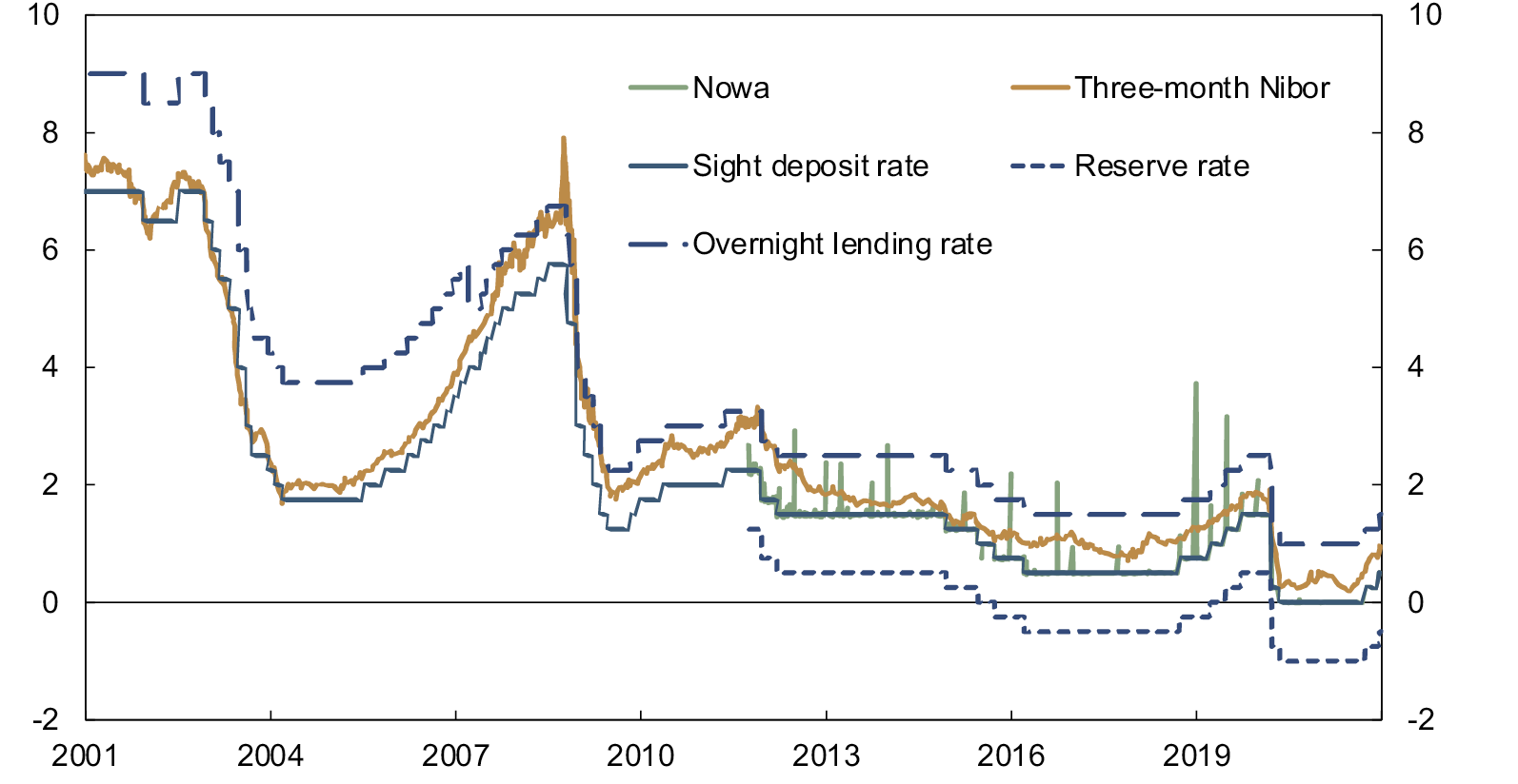
Sources: Bloomberg and Norges Bank
Forward guidance
The policy rate influences the interest rates banks, households and businesses face from day to day. When economic agents make decisions, however, expectations about future developments in the policy rate play a role. An important part of monetary policy is therefore to manage expectations about developments in monetary policy. There are a number of ways to engage in such expectations management.
Norges Bank has published policy rate forecasts, the policy rate path, since 2005. Norges Bank’s policy rate path expresses the interest rate that in the Bank’s opinion provides the best possible trade-off between monetary policy objectives. The rate path shows the Bank’s expected developments in the policy rate, given its current assessment of the state of the economy, outlook, balance of risks and functioning of the economy. The policy rate forecast is shrouded in considerable uncertainty. If the economic outlook, balance of risks or the Bank’s assessment of the functioning of the economy change, the policy rate may also turn out differently from the one indicated by the rate path.
With the aid of the policy rate paths and related communication, Norges Bank provides forward guidance regarding future policy rate developments and information about the central bank’s response pattern. When these signals are perceived as credible, the effect of future changes in the policy rate may occur earlier.
Norges Bank attaches weight to transparency in its monetary policy communication. The aim is for the decision basis and trade-offs on which a monetary policy decision is based to be reflected in the MPR. The MPR provides more information about trade-offs, assessments and the outlook than most similar reports by other central banks, where trade-offs and monetary policy assessments are more commonly reflected in the minutes of decision-making meetings.
Central bank communication is constantly evolving. During the GFC, a number of central banks ended up in a situation where their ability to conduct conventional monetary policy was limited by the lower bound for the policy rate. Unconventional measures (see Section 3.5) were employed, such as asset purchases (quantitative easing) and what has been called “forward guidance”. At the time, the term forward guidance was used for explicit statements by the central bank on future policy rate developments. While the aim of monetary policy in normal times had been to enhance the effectiveness of monetary policy instruments, the purpose of forward guidance was for central bank communication itself to become a monetary policy instrument.62 Since the GFC, forward guidance has evolved into a broader and more normal concept.63 Today, the policy rate path and Norges Bank’s statements on future policy rate developments are referred to as the central bank’s forward guidance.
Two types of forward guidance are often distinguished in the literature. In one variant, the central bank issues a statement on future policy rate developments, given its economic assessment. This type of forward guidance can be viewed as pure forecast, and not a promise. Norges Bank’s policy rate path is an example of this type of forward guidance. In the other variant, there is more of a commitment by the central bank to a specific monetary policy within a certain horizon or dependent on certain economic conditions. This type of forward guidance is therefore more akin to a promise than a forecast; the central bank seeks to influence expectations by “tying itself to the mast”. That is why the former type is often referred to as “Delphic forward guidance”, while the latter type is called “Odyssian forward guidance”. In practice, communication about future monetary policy will often have elements of both types of forward guidance.
Odyssian forward guidance may be particularly useful in a crisis situation or when the policy rate is close to its lower bound. An example is when the US Federal Reserve announced in 2012 that its policy rate would be held close to zero as long as unemployment was above 6.5 percent, provided that inflation did not rise significantly in the meantime.
60 The policy rate and the implementation of monetary policy are described further in Norges Bank (2021).
61 Central bank reserves serve as means of interbank settlement: When a bank deposit is transferred from Bank A to Bank B, reserves are transferred from Bank A’s account in the central bank to Bank B’s. A bank is willing to accept customer deposits from other banks (liabilities) because at the same time an equal amount of central bank reserves (a claim on the central bank) is transferred to its reserve account. This enables banks’ customers to use their deposits as a means of payment to customers of other banks.
62 See Issing (2019), page 38.
63 “Departing from the zero lower bound will deprive forward guidance of its special necessity as the only remaining monetary policy instrument. In the end, the term ‘forward guidance’ might remain, but the meaning will be reduced to the state of normal communication to guide expectations with the aim of making monetary policy more effective.” Issing (2019), page 38.
Norges Bank’s principles for liquidity policy and the role of the central bank1
One of the aims of liquidity policy is to keep the shortest money market rates close to the policy rate. The central bank achieves this by setting the terms for banks’ loans and deposits in the central bank and by controlling the quantity of central bank reserves in the banking system (referred to as the liquidity management system). In addition to ensuring the implementation of monetary policy, the aim of liquidity policy is to promote an efficient payment system and financial stability. Liquidity policy also plays an important role in times of financial stress in that the central bank can inject liquidity into the banking system or provide loans to individual banks on special terms.
There are different types of liquidity management systems, all of which regulate the supply and cost of central bank reserves. The most common are variations of what are known as corridor and floor systems. In a corridor system, banking system reserves are low (at zero or marginally above zero) and the policy rate is normally midway between the Bank’s deposit and lending rates for banks, referred to as the standing facilities. Such a system gives banks an incentive to borrow from and deposit reserves with each other overnight. Otherwise, banks with a positive balance on their account with the central bank have to deposit these reserves at the deposit rate (which is lower than the policy rate), while banks with a negative balance have to borrow reserves from the central bank at the lending rate (which is higher than the policy rate). The purpose of the interest rate corridor is to give banks an incentive to avoid using the central bank’s standing facilities, but instead redistribute the reserves among themselves in the interbank market at a rate close to the policy rate. In a floor system, on the other hand, the central bank ensures there is an ample supply of reserves in the banking system. As a result, the overnight interbank rate is pushed down towards the central bank deposit rate, which will then be the policy rate. Compared with a corridor system, it is cheap for banks to keep reserves at the central bank under a floor system because all reserves are remunerated at the policy rate.
Norges Bank uses a quota system in its liquidity management. In a quota system, a certain quantity of banks’ reserves is remunerated at the policy rate, ie a quota. Deposits in excess of the quota are remunerated at a lower interest rate, the reserve rate. This means that banks have an incentive to keep deposits below the quota. If the deposits are likely to exceed the quota, banks then have an incentive to lend reserves in the interbank market, in the same way as in a corridor system.
In a quota system, as in a corridor system, keeping large reserves at the central bank is costly for banks as deposits in excess of the quota are remunerated at a rate below the policy rate. In a quota system, central bank reserves are primarily intended in normal times to serve as a means of settlement between banks rather than a store of value. This is in line with Norges Bank’s principles for liquidity policy, where the objectives are: (1) ensure that there is a high degree of pass-through from Norges Bank’s policy rate to money market rates, (2) promote an efficient payment system, (3) offer liquidity insurance and act as lender of last resort, and (4) provide a framework for liquidity and credit risk to be borne as far as possible by private agents in the financial system. The first three objectives can also be achieved in a system with an ample supply of reserves (such as a floor system). However, if it is important for risk to be borne by private agents (4), it must cost more to keep central bank reserves as a liquid asset of durable value.
The objective that risk should be borne by private agents reflects the low level of risk tolerance the central bank should have. If banks can borrow substantial reserves from the central bank at a low price, the central bank’s role in transforming securities pledged as collateral for loans into highly liquid assets (central bank reserves) entails the transfer of considerable risk from the banking system to the central bank. The central bank’s risk will be low if the securities’ credit risk is low and haircuts are applied to their collateral value. In practice, however, it is difficult for the central bank to fully eliminate this risk. The more reserves the central bank must offer banks in the form of loans, the higher the central bank’s potential exposure to credit risk will be.
The principle of sharing risk between private agents and the central bank also reflects the regulatory liquidity and capital requirements imposed on banks by the authorities. The authorities’ requirements are largely intended to ensure that banks must adjust their balance sheets so that they are resilient to substantial risk without needing liquidity support from the central bank or other public authorities. As little risk as possible should be transferred to the central bank in particular or to the government in general. The central bank’s liquidity policy should support this principle, ie contribute to ensuring that risk is borne by the private banking system.
In line with this view, central bank reserves should primarily be a means of settlement for banks and thereby a liquidity management instrument that ensures the efficiency of the payment system and the efficient transmission of monetary policy. In times of financial market stress, when central bank measures can involve offering substantial central bank reserves that are then used as a store of value, the reserves offered should be priced separately and not be a consequence of the ordinary conduct of liquidity policy.
1 Based on Norges Bank (2021).
3.1.2 Transmission mechanism
When the central bank changes its policy rate, the real interest rate will be affected because prices are sticky in the short and medium term. In an open economy, policy rate changes will also affect the nominal and real exchange rate. These effects pass through to the economy through several channels. The transmission mechanism is a blanket term that covers the policy rate’s pass-through channels, and it is common to distinguish three primary channels: the demand channel, the exchange rate channel and the expectations channel.
- The demand channel describes how a change in the policy rate affects total demand and hence inflation. A change in total demand will affect inflation through changes in price and wage inflation. A reduction in total demand will reduce demand for labour, thereby pulling down wage inflation. At the same time, inflation will be pulled down when firms’ reduce the rise in prices for the goods they sell. The effect of the policy rate on total demand can be divided into four elements:
- Interest rate channel to total demand: A change in the real interest rate will affect total demand in the economy by influencing consumption and investment. An increase in the real interest rate makes saving more attractive, at the same time as households’ borrowing costs rise. This reduces household demand for consumption goods. Firms will thus experience lower demand for the goods they sell and at the same time face higher investment costs. This reduces investment demand.
- Wealth channel to consumption: An interest rate increase reduces the value of net household wealth, thereby reducing household demand for goods and services. A change in the interest rate affects financial asset prices, but also the value of housing wealth. For Norwegian households, the wealth effect of house prices will be the most pronounced wealth effect.
- Cash flow channel64 to total consumption: A higher interest rate will also reduce the disposable income of households with net debt, giving rise to a cash flow channel that will reduce demand further from households with net debt, as is the case for the average Norwegian household. For households with limited liquid funds facing borrowing constraints, the cash flow channel can have a pronounced impact on consumption. A fall in house prices as a result of an interest rate increase makes it more difficult for households to borrow against home equity. This can also contribute to lower consumption demand.
- Exchange rate channel to total demand: A movement in the exchange rate will affect total demand by affecting net exports. An increase in the policy rate will, in isolation, pull in the direction of a stronger krone. This makes our exports more expensive and contributes to a reduction in net exports.
- The exchange rate channel to inflation describes how a stronger krone resulting from a policy rate increase will make imported goods cheaper and lead to lower imported inflation, in turn contributing to lower consumer price inflation.
- The expectations channel describes how expectations of a future interest rate affect total demand and inflation. The policy rate is an overnight interest rate, which in itself is not of particular importance for demand and inflation. It is the money market rates and banks’ deposit and lending rates that matter, and these rates are largely determined by economic agents’ expectations of future levels of the policy rate. The central bank influences agents’ expectations through forward guidance. This guidance can be in the form of statements, eg that the policy rate will most likely be raised in the course of the next six months, or in the form of policy rate forecasts, which Norges Bank and some other central banks publish.
See “How the policy rate influences the Norwegian economy” for more about the functioning of the transmission mechanism in the Norwegian economy.
It is widely assumed that monetary policy only has a transitory effect on the economy, ie it is neutral in the long run. In the short (and medium) run, monetary policy may affect real economic variables such as output and employment. But further out, the effect of monetary policy will fade, with variables returning to their equilibrium levels. Monetary policy is capable of influencing nominal variables in both the short and long run.
To the extent that economic fluctuations are asymmetric, eg owing to labour market hysteresis, monetary policy can, in principle, contribute not only to reducing variability in output and employment but also to raising the averages of these two variables. See Section 2.2 for a further discussion of this effect.
64 See Gerdrup and Torstensen (2018) for a static analysis of the cash flow channel.
How the policy rate influences the Norwegian economy
Looking at the impulse response functions of a monetary policy shock in NEMO gives us a picture of how the transmission mechanism functions in the Norwegian economy. Chart 1 presents the impulse response functions for a sample of macro variables: inflation, output, exchange rate, policy rate, house prices and wage growth.1 We look at a shock that is normalised so that the policy rate rises at most by 1 percentage point on an annualised basis.
Chart 1 Impulse response functions of a monetary policy shock in NEMO
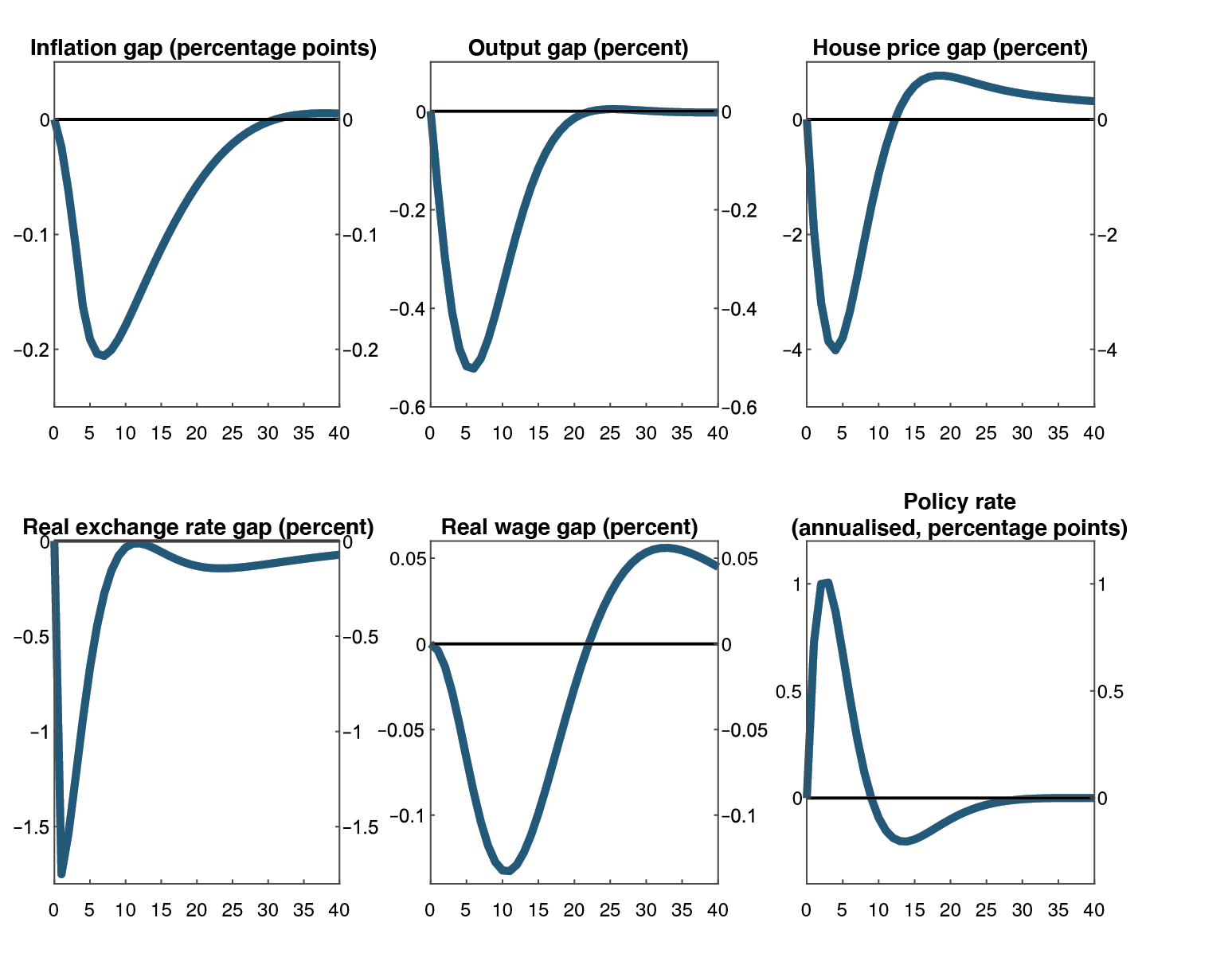
In the model, a change in the policy rate affects the economy through the demand channel, exchange rate channel and expectations channel. A policy rate hike results in a reduction in domestic demand and a stronger real exchange rate. The rise in short-term interest rates affects the real economy through the banking sector. A rise in lending rates to households and businesses depresses household consumption and business investment, leading in turn to a fall in total demand and thus in total output. A fall in house prices amplifies the decline in consumption and investment and limits households’ additional borrowing, since borrowing depends on home values. In addition, a stronger exchange rate reduces exports and leads to a shift from domestically produced goods to imports. It takes a little over a year before the effect on output is at its most pronounced, at which time output is around 0.5 percent lower than it would have been absent the policy rate hike.
As a consequence of the fall in total demand, non-financial businesses will reduce their demand for labour, which will lead to a decline in wages and number of hours worked. This reduces the prices of domestically produced goods. In addition, a stronger exchange rate pushes down import prices. It takes a little over two years before the effect on inflation is at its most pronounced, at which time inflation is 0.2 percentage point lower than it would have been absent the policy rate hike.
In Chart 1, we see that the effect of a policy rate hike on total demand does not completely fade until after four years, while the effect on inflation persists for six years. It is important to note that the impulse responses only show the isolated effects of the monetary policy shock. In reality, the economy will be hit by new shocks in the meantime, and the central bank’s ability to control inflation and output will thus be far from perfect.
1 See Kravik and Mimir (2019) for impulse response functions for more variables.
3.2 Decision basis
Norges Bank’s decision basis for monetary policy is founded on analyses and forecasts of the Norwegian and global economy. These analyses and forecasts are updated four times a year and are published in the Bank’s monetary policy report (MPR). They are based on assessments of the current situation, projections for exogenous variables, ie variables that are not, or are to a limited extent, affected by Norges Bank’s policy rate setting, over the entire forecast horizon (for example public demand), a quantification of relationships in the economy in both the near and long term and our perception of these relationships. In our forecasting, we seek to build a bridge between the assessment of the current situation and our assumptions regarding the long-term relationships in the economy. In addition, the forecasts are determined by the Monetary Policy and Financial Stability Committee’s trade-offs between monetary policy objectives. When the fundamental premises change, the projections for developments in the policy rate (the policy rate path) and other economic variables will also change.
In order to project future economic developments, we need to have a thorough analysis of the current economic situation. The analyses of the current situation are based on updated statistics and other information about cyclical developments. Together with assumptions regarding exogenous driving forces, ie driving forces considered to be independent of monetary policy in Norway, the analyses form the basis of our monetary policy analysis and forecasts (Chart 3.2). This results in a decision on what the policy rate should be set at now and our forecast of policy rate developments ahead, in order to best attain the Bank’s monetary objectives. Monetary policy trade-offs are discussed further in Section 2.4.
Chart 3.2 The system for monetary policy analysis and forecasting
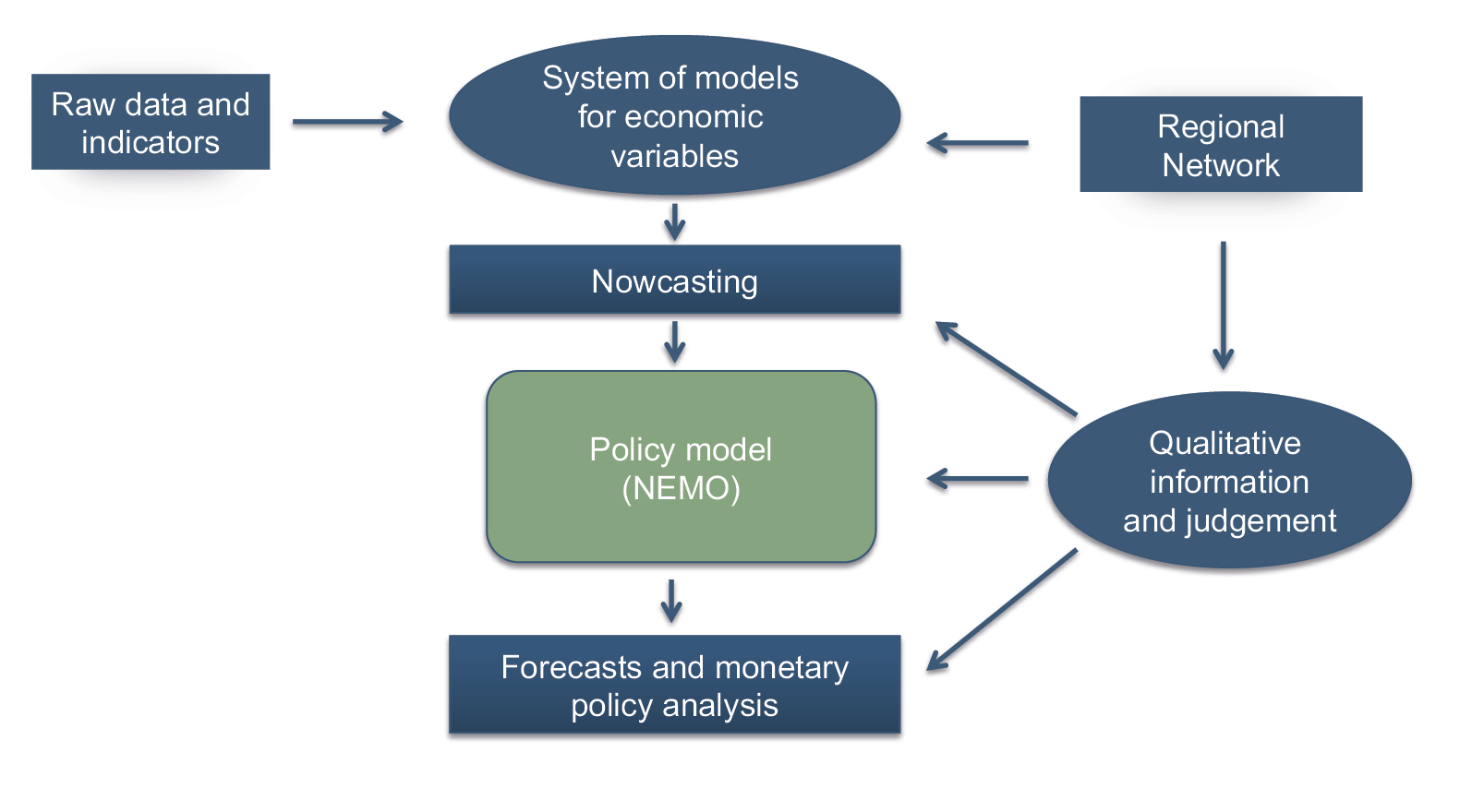
Regional Network
In 2002, Norges Bank established a regional network of around 1500 enterprises, organisations, local governments, hospitals and other public bodies throughout Norway. Four times a year, management-level contacts in around 300 of these enterprises and organisations are interviewed about economic developments and the outlook ahead.
The contact sample reflects the production side of the economy both by sector and geographically. Norges Bank's Regional Network is divided into seven regions: North, Central, North-West, South-West, South, Inland and East. Norges Bank has primary responsibility for the network as a whole and for Region East, while regional research institutions gather information from the rest of the country.
The purpose of the network is to obtain early signals of developments in the Norwegian economy. Regular interviews with contacts give Norges Bank timely and useful information about contacts’ assessments of the current situation and the outlook for their own business or institution.1 The responses are summarised in reports and data series for key economic variables at the national, regional and sector level.
Direct contact with executives enables the Bank to obtain nuanced and comprehensive information that is not covered by statistics or captured in a questionnaire. For that reason, both qualitative and quantitative information from network contacts is actively used in the Bank’s analyses and forecasting and thus form part of the basis for monetary policy decisions.
Information from the network has proved to provide a reliable indication of Norwegian economic developments over time (Chart 1).2 Regional Network data for actual and expected growth in output and employment provide reliable estimates of output and employment growth in the national accounts one to two quarters ahead.
The results from the Regional Network are judgement-based assessments based on interviews of network contacts. Reports from the Regional Network do not represent the views of Norges Bank or individual enterprises on economic developments.
Chart 1. GDP for mainland Norway1 and Regional Network indicator for output growth2
Quarterly change. Percent. 2013 Q1 – 2022 Q13
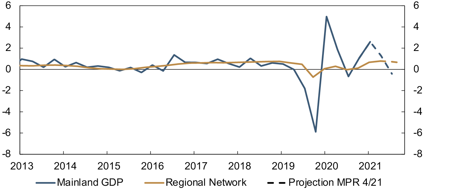
1 Seasonally adjusted.
2 Reported output growth over the past three months converted to quarterly figures. Quarterly figures are calculated by weighting three-month figures on the basis of survey timing. For 2022 Q1, a weighting of historical and expected growth is used, while expected growth is used for Q2.
3 Projections for 2021 Q3 – 2022 Q1
Sources: Statistics Norway and Norges Bank
1 The Regional Network's samtaleguide (pdf) (interview guidelines, in Norwegian only) contain a list of the main topics discussed.
2 See Brander, Brekke, Naug and Eger (2017).
3.2.1 Data and information sources
In order to make sound monetary policy trade-offs and accurate forecasts, Norges Bank depends on reliable data and information on economic developments in Norway and abroad. Norges Bank therefore obtains a broad set of data from different statistics providers.
Norges Bank analyses economic developments among Norway’s trading partners. In addition to data from global financial markets and developments in interest rates and interest rate expectations, the Bank monitors in particular data on output, employment and prices. The Bank also closely monitors energy and commodity markets, using for example reports from international organisations such as the International Energy Agency (IEA) and the US Energy Information Administration (EIA).
Statistics Norway is an important source of data for Norway. The consumer price index (CPI) is one of the most important variables in the monetary policy analysis. Norges Bank closely monitors consumer prices adjusted for tax changes and excluding energy products (CPI-ATE) and other underlying inflation indicators produced by Statistics Norway. The Bank also estimates a number of underlying inflation indicators (see “Indicators of underlying inflation”). The broad range of inflation indicators help provide a more detailed picture of underlying inflationary pressures.
Main economic aggregates in the national accounts are key to understanding cyclical developments in the Norwegian economy. Total gross domestic product (GDP) is an important main aggregate, but because the business cycles have little influence on petroleum production, we give particular weight to mainland GDP, where oil and gas extraction, pipeline transport and international shipping are excluded. Both the production and demand side of the economy are analysed to understand the driving forces behind economic developments. Demand components, such as household consumption, business investment, housing investment, petroleum investment, public demand, exports and imports are analysed in detail to gauge the current situation in the economy and project future economic developments. Household income accounts provide important additional information on household consumption and saving behaviour.
Statistics Norway is also an important source of insight into the labour market. The national accounts provide information on employment developments in Norway, while the Labour Force Survey (LFS) estimates the size of the labour force, employment and unemployment. The Norwegian Labour and Welfare Administration (NAV) is also a key provider of labour market data and publishes monthly data on registered unemployment, in addition to data on eg unemployment benefit applications, furloughs, redundancies and job vacancies.
Statistics Norway’s register statistics on the number of jobs and wages provide further information on employment developments and are a key source of information on current wage developments through the year. Reports from the Technical Calculation Committee for Wage Settlements (TBU) on the basis for wage settlements provide important information on for example wage carryover in sectors affected by wage agreements and the social partners’ inflation expectations.
Public documents such as the National Budget and the Report to the Storting on Long-Term Perspectives for the Norwegian Economy provide insight into the fiscal policy stance and are useful in assessing the outlook for public demand. Projections for increases in tax revenues and transfers in public documents are included in the basis for Norges Bank’s projections for household disposable income and consumption.
Norges Bank’s Regional Network collects information from a broad sample of businesses across Norway (see “Regional Network” for further details). The Regional Network provides the Bank with both quantitative and qualitative information, which is useful when interpreting statistics and improves the Bank’s understanding of economic developments. The information from Regional Network contacts also functions as a cross-check of early statistics that are uncertain and are often subsequently substantially revised. The Expectations Survey, conducted by Ipsos on behalf of Norges Bank, provides information on expectations of price and wage inflation, for example.
In the event of very sudden and sharp shocks to the economy, alternative data sources may be particularly useful. In recent years, Norges Bank has used a number of new data sources to monitor developments in real time. Card transaction data have been particularly useful in the assessment of consumption and saving behaviour during the Covid pandemic. Mobility and search data from the technology company Google have also provided timely and frequent information on household behaviour through the pandemic. The use of such data changes continually as new technology increasingly enables new and faster data sources to be utilised.
New technology also makes it possible to process ever larger amounts of data at a lower cost. Individual- and firm-level data are important in the Bank’s work to achieve a deeper understanding of important economic mechanisms. Microdata from the a-ordning (a coordinated service used by employers to report income and other employee information to NAV), the tax authorities and various registers improve the Bank’s understanding of different groups’ movements in and out of the labour market. Data on all firms in Norway help to ascertain and understand the risk of bankruptcy and possible spillovers.
The information base we use when preparing our projections for developments in Norway and abroad also contains analyses from the International Monetary Fund (IMF), the Organisation for Economic Co-operation and Development (OECD), other central banks and investment banks. Projections from Norwegian and international institutions function as a cross-check of Norges Bank’s forecasts.
The analyses in the MPR are normally based on information up to and including the Friday before publication of the MPR and the interest rate decision. The monetary policy decision is based on information up until the decision is made.
3.2.2 Models and use of models
Norges Bank utilises a spectrum of models in order to answer different questions. For short-term forecasts of the economy, we primarily use empirical models with the best possible forecasting properties. Medium- and long-term projections are based more on models constructed using economic theory that are calibrated and estimated to capture the transmission mechanisms from monetary policy to economic variables.
Short-term projections and exogenous forecasts
Norges Bank’s System for Averaging short-term Models (SAM)65 is used for short-term projections of inflation and GDP. In SAM, projections from different empirical model classes are combined. The projections are weighted together on the basis of their historical forecasting capabilities.
Moreover, and for other aggregates, a broad spectrum of empirical models is used to forecast economic activity in the short term.66 Some exogenous variables are forecast outside the Bank’s modelling system. The term “exogenous” is used for factors normally thought to be unaffected by Norwegian monetary policy. Examples of exogenous variables that are forecast are foreign inflation and output, and money market premiums. Forecasts for oil prices and future interest rates among trading partners are based on market expectations. Forecasts for public demand usually follow a technical assumption based on the National Budget and other public documents.
In order to forecast foreign inflation and output, a combination of internally and externally produced models are used, both short-term and potential growth models. The Bank is part of the IMF Global Projection Model Network (GPMN) and uses the GPM model as a consistency check for projections two to three years ahead. The GPM is also used to make scenario analyses, along with the Global Integrated Monetary and Fiscal Model (GIMF), also developed by the IMF.
Empirical cross-check models
As well as having a wide array of models to project short-term developments, Norges Bank has developed empirical models that are used to cross-check the projections from the Bank’s main model, the Norwegian Economy Model (NEMO). The models are Bayesian VAR models and contain many of the same variables as NEMO. In a projection process, iterations are made between the cross-check models and NEMO.
Norges Bank is further developing the SAM system to include new model classes, extend the projection horizon and increase the number of variables included. The main purpose is to combine all empirical models in a single model framework (SMART – System for Model Analysis in Real-Time) and effectively utilise newly developed empirical models in forecasting.
NEMO – Norges Bank’s macroeconomic main model
Norges Bank’s macroeconomic main model NEMO is used as the basis for monetary policy analyses but also to provide forecasts of economic variables in the medium and long term.67 Moreover, the model is a useful tool in the work to understand the underlying forces driving economic fluctuations. The model has been in continuous development since it was first used in 2006.
NEMO is a dynamic, stochastic, general equilibrium (DSGE) model for a small open economy and shares features with macroeconomic models at other central banks. NEMO models the behaviour of households, firms, private banks and the central bank. The task of monetary policy in the model is to help to stabilise the economy and bring inflation back to target when the economy has been exposed to shocks. The model contains a Norwegian and a foreign sector, where the Norwegian oil services industry is a separate production sector. The foreign sector is assumed to affect the Norwegian economy, but the converse is not the case. This is a common assumption in small open economy models.
In models such as NEMO, developments in endogenous variables (those determined in the model) will depend on exogenous variables (those determined outside the model). The endogenous variables will fluctuate around a long-run equilibrium level that is determined by structural conditions in the Norwegian economy. Since the equilibrium level cannot be observed, statistical methods and judgement are used to estimate equilibrium levels on the basis of historical data. NEMO interprets the history and the projections and finds the combination of shocks that explains with the greatest degree of probability the fluctuations around the estimated equilibrium levels. These shocks will typically operate through numerous channels and affect the economy for a lengthy period.
On the basis of its interpretation of economic driving forces and shocks, the model generates a policy rate forecast based on minimising a loss function (see “Modelling objectives and trade-offs: Loss functions”). The model generates a policy rate path that brings inflation back to target and closes the output gap. In order to obtain the best possible projection, we condition NEMO on short-term projections and forecasts for exogenous variables.68
The policy rate forecast generated by the model serves as input into the monetary policy discussion. What constitutes a reasonable trade-off in monetary policy is judgement-based (Section 2.4). There is no mechanical link between the model’s policy rate path and Norges Bank’s policy rate forecasts. Even so, such models can provide the monetary policy analysis with a fundamental structure and discipline the monetary policy discussion.
Norges Bank will continue working to improve the model,69 including by following up on advice from an expert committee that has evaluated Norges Bank’s macroeconomic models.70 Work is in progress to incorporate more realistic expectations formation into NEMO, and a more long-term objective is to incorporate more macroeconomic trends into the model. As the expert committee pointed out, simplifying parts of the model may be relevant. Moreover, in order to have a more flexible framework for analysing the monetary policy implications of alternative assumptions in the model, a smaller macroeconomic model is also in development. This model will be quantified based on the Norwegian economy in the same way as NEMO. There is also a focus on constructing a modelling system featuring heterogeneous agents that can improve our understanding of household consumption and saving behaviour and the effect of the policy rate on these decisions. This work is supported by empirical analyses based on microdata for households, including transaction data, income and wealth. We will also investigate how our analysis and modelling system can best take account of physical climate change and climate adaptation effects both globally and in Norway on the Norwegian economy.
Judgement
Judgement, qualitative information and expertise are used at all stages of the decision-making process, for assessing the economic situation, for producing projections and for assessing monetary policy. New relevant information and new assessments rarely point in the same direction. The forecasting process is therefore largely iterative.
3.2.3 Evaluation and quality assurance
Norges Bank attaches importance to transparency in its monetary policy communication. The Bank reports on the conduct of monetary policy in its Annual Report. The trade-offs on which policy rate setting are based are published regularly, including in the MPR.
Norges Bank’s projections of economic developments, both in Norway and among our main trading partners are evaluated annually. Evaluating and analysing our forecasting errors enables us to increase our understanding of the functioning of the economy and improve our forecasts. The evaluations are published in the series Norges Bank Papers, usually annually.71
Norges Bank Watch (NBW) is an independent expert group that has evaluated the conduct of monetary policy each year since 2000.72 The composition of the NBW group varies from year to year. The members are appointed by the Centre for Monetary Economics (CME) at BI Norwegian Business School. The purpose of NBW is to contribute to the debate on Norwegian monetary policy and provide input to the public on both how Norges Bank has defined its role and how its policy is implemented and communicated to the outside world.73
NBW reports serve inter alia as input to the Ministry of Finance’s evaluation of Norges Bank’s conduct of monetary policy.74 The Ministry’s assessment is presented to the Storting (Norwegian parliament) in the annual Financial Markets Report, and the governor appears in a public hearing before the Standing Committee on Finance and Economic Affairs in connection with the debate on the report.
65 SAM is described further in Aastveit, Gerdrup and Jore (2011). See also the discussion on challenges posed by the SAM system during the pandemic in the box “Unusually high forecast uncertainty” on page 40 of MPR 2/2020.
66 These models are formulated in a reduced form. The modelling system consists of VAR models, factor models and single equation models, and are used both to produce projections, but also to gain a better understanding of economic drivers.
67 The model is described further in Kravik and Mimir (2019).
68 The forecasts are cross-checked against the forecasts of a range of other models at sectoral level. Smaller theoretically based DSGE models complement NEMO in conceptual matters, and Norges Bank is working on developing models that are based on microdata and incorporate irrational behaviour.
69 See the Special Features “Macroeconomic model NEMO – mechanisms and driving forces” in MPR 3/17 and “Re-estimated version of NEMOˮ in MPR 4/18
70 See Canova, Furlanetto, Smets and Wieland (2019).
71 See eg Re-estimation for 2017.
72 See the reports from NBW.
73 See Chapter 6.2.10 of NOU (Official Norwegian Report) 2017:13.
74 Since 2001, the Ministry of Finance has contributed towards the financing of the reports from NBW.
3.3 Neutral monetary policy and indicators of monetary tightness
In order to assess whether monetary policy is expansionary or contractionary, a “zero point” is needed, where the effect of monetary policy on demand in the economy is neutral. It is not obvious how “neutral monetary policy” should be defined, but the most common measure is the “neutral real interest rate”75. It is defined as the level of the real interest rate that is neither expansionary nor contractionary. The neutral real interest rate is thus a key concept for assessing monetary tightness. As we cannot observe the neutral real interest rate, estimations of it will be uncertain.
3.3.1 Literature and international practice
The term was introduced by Wicksell (1898), who defined the neutral real interest rate as the interest rate that is consistent with stable developments in commodity prices. In Wicksell’s view, the general price level would rise or fall as long as the real interest rate deviated from the neutral real interest rate. The concept was subsequently formalised and developed further in Woodford (2003). Here the neutral real interest rate was defined as the rate that would arise in an economy without nominal rigidities, ie where prices and wages are fully flexible. In Woodford’s definition, any shock regardless of duration will affect the neutral real interest rate, something that could potentially entail wide fluctuations in the neutral real interest rate even in the short term.76
In other words, the various definitions of the neutral real interest rate in the literature differ primarily with regard to the persistence of the shocks included. In the conduct of policy, there is good reason to disregard factors regarded as transitory in a definition of the neutral interest rate. Transitory shocks are demanding to identify in real time, and a measure of the neutral real interest rate that differs widely from one quarter to the next is not suitable as a reference point for monetary policy. It is especially important to distinguish the neutral real interest rate from what we call the long-run equilibrium interest rate. The long-run equilibrium interest rate is determined by fundamental economic factors, such as potential growth and consumers’ saving behaviour. However, the neutral real interest rate is also determined by various shocks that affect the supply and demand sides of the economy in the medium run. In the long run, the neutral real interest rate will correspond to the equilibrium interest rate in the economy, while it may deviate from it in the short and medium run. In a world of high capital mobility, it is reasonable to assume that the long-run equilibrium interest rate will be a global variable.77
Long-term global interest rates have shown a clearly falling trend since the mid-1980s (Chart 3.3). The decline in the first part of the period reflects lower actual and expected inflation. In the past decades, most of the decline in nominal interest rates is probably the result of the decrease in real interest rates. As it is unlikely that monetary policy can influence the real interest rate over time, developments must primarily be interpreted as a fall in the neutral real interest rate.
Central banks differ in their practices in publishing their estimates of the neutral real interest rate. The Bank of Canada (BoC) reviews its estimates of the neutral real interest rate every year and uses various approaches to arrive at its estimates. In 2021, the BoC revised down the neutral nominal interest rate in Canada78 to lie in the range of 1.75 to 2.75 percent.79 The US Federal Reserve has not explicitly defined the neutral interest rate80, but the median of FOMC members’ projections for the federal funds rate over the long term is often regarded as a possible estimate. Various estimation methods suggest that the long-term neutral nominal interest rate in the US may lie in the range of 2.5 to 3.5 percent.81 The neutral real interest rate in the euro area is estimated to have been around zero or negative in recent years.82
Chart 3.3 Yields on 10-year government bonds1. Percent. 1980–2021
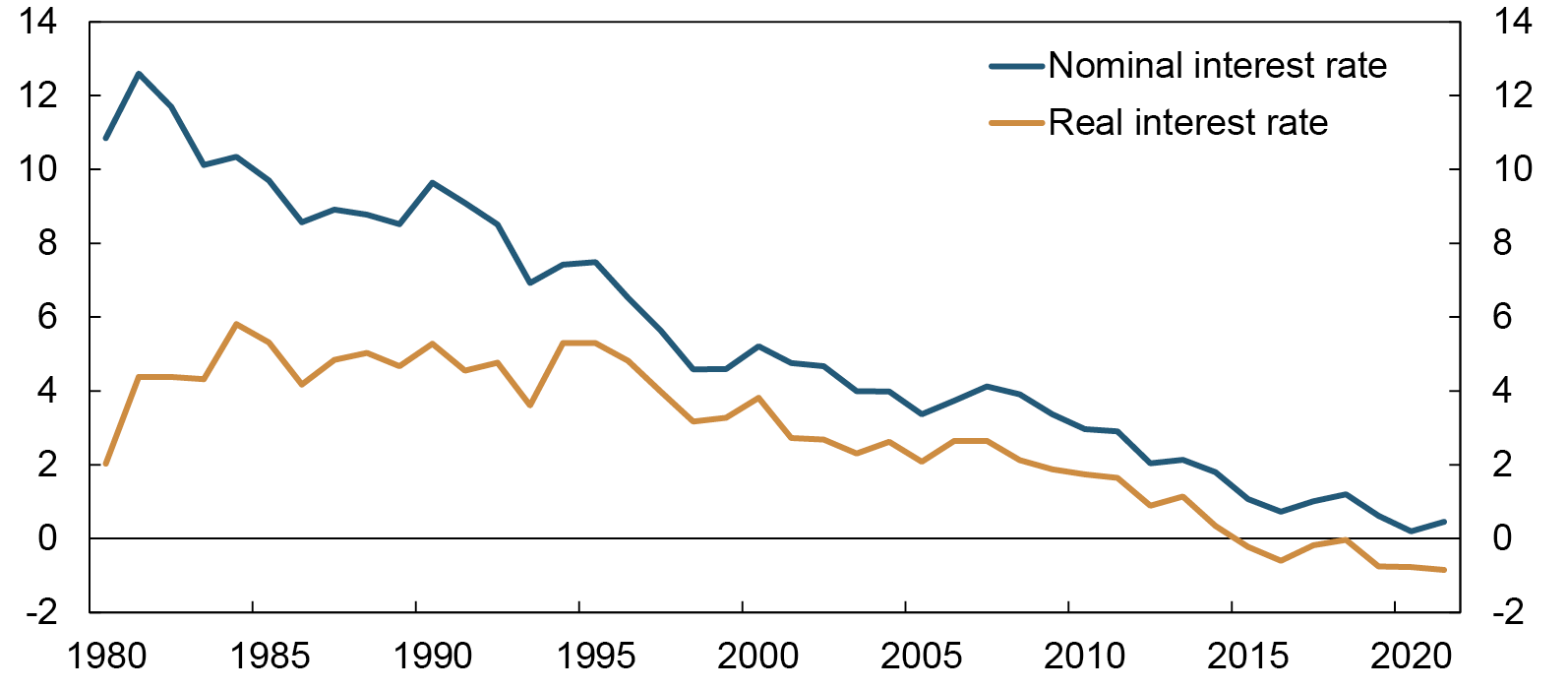
1 The following countries are included in addition to Norway: Austria, Belgium, Canada, Denmark, France, Germany, Italy, Japan, the Netherlands, the UK, Switzerland and the US. Unweighted average. Real interest rate is nominal interest rate less average inflation in current year.
Sources: Refinitiv datastream and Norges Bank
One objection to exclusively regarding the deviation between the actual real interest rate and the neutral real interest rate as an indicator of monetary tightness is that it does not capture other financial conditions, such as credit standards, credit supply, asset prices and the exchange rate. The importance of the different factors can vary across countries owing to differences in the financial system and participants’ funding structures. The nominal interest rate can also have an impact over and above the real interest rate as it affects households’ and businesses’ cash flows. Financial conditions also affect demand and can be regarded as part of monetary policy in a broader sense.
An alternative method of measuring monetary tightness is a Financial Conditions Index (FCI). Movements in financial variables are often not synchronous, and the macroeconomic impact of changes in one variable can be offset by another. While an increase in the money market rate will normally signal tighter financial conditions, the overall effect can be reversed if banks’ credit standards are eased at the same time or the price of risk falls in securities markets. The aim of an FCI indicator is to summarise the effect of changes in various financial variables and make it easier to interpret the macroeconomic effect of these changes. FCI indicators are used actively by many countries’ central banks, institutions and major banks.83 An FCI for Norway is being developed by Norges Bank.84
3.3.2 Norges Bank’s interpretation of the neutral real interest rate
Norges Bank has chosen to define the neutral real interest rate as the rate consistent with balanced economic developments in the medium term when the impact of transitory shocks has unwound (normally within five to ten years). Balanced economic developments refer to output in line with potential output and inflation at target. The neutral real interest rate, according to this definition, is primarily determined by structural conditions. In a small open economy such as Norway, underlying conditions are influenced to a great extent by international developments. This means that the neutral real interest rate in Norway will likely remain close to the global neutral real interest rate over time.
In MPR 2/21, the neutral real money market rate was assumed to be around zero. Norges Bank uses both economic models and market-based measures to estimate the neutral real interest rate. The various estimates all indicate a persistent 3–5 percentage point decline in the neutral real interest rate over the past 20 years. See “Norges Bank’s estimates of the neutral real interest rate”.
75 The terms “neutral real interest rate”, “natural real interest rate” and “normal real interest rate” are used interchangeably in the literature. In this paper, the term “neutral real interest rate” is used.
76 See Brubakk, Ellingsen and Robstad (2018).
77 See Bernhardsen and Gerdrup (2006).
78 Defined as the neutral real interest rate plus the inflation target.
79 See Brouillette et al (2021).
80 The Federal Reserve Bank of New York publishes updated estimates of the neutral real interest rate as estimated in Laubach and Williams (2003) and Holston, Laubach and Williams (2017).
81 See Brainard (2018).
82 See Lane (2019).
83 See Alsterlind et al. (2020) for an example from Sveriges Riksbank and references to other institutions producing FCIs. Jensen and Pedersen (2019) analyses financial conditions in Denmark.
84 See Vonen (2011) for a previous Norges Bank analysis.
Norges Bank’s estimates of the neutral real interest rate1
Norges Bank uses a range of methods to estimate the neutral real interest rate. Model estimates are now used in addition to purely market-based measures. Long-term market rates provide an indication of market expectations of future interest rates. As the effects of past transitory shocks to the economy can be expected to unwind in the course of five to ten years, it can be assumed that their effect on long-term interest rate expectations is limited. Adjusted for expected inflation, implied long-term interest rate expectations can express market estimates of the neutral real interest rate.
The model estimates are based on two types of empirical model, two vector autoregressive (VAR and BVAR) models and different state-space (SS) models. The models mainly differ in their degree of theoretical foundation.
The VAR model is a purely statistical model with time-varying parameters.2 The model is based on the interplay between output, inflation and the real interest rate, but includes time variation in these relationships. The neutral real interest rate is defined as the model’s current estimate of the actual real interest rate five years ahead.
The Bayesian VAR model (BVAR) is also a purely empirical model, where the underlying trend (the deterministic component) in the nominal interest rate and inflation are used to estimate a trend for the real interest rate.
The SS models rely to a greater extent on economic theory.3 In these models, there is a direct relationship between the level of capacity utilisation in the economy and the difference between the actual and the neutral real interest rate (IS curve). Capacity utilisation in turn affects inflation via the Phillips curve4.5 The neutral real interest rate depends on both potential output and other unspecified factors that influence saving and investment decisions. Based on data and the assumed relationships, the most likely historical path of the neutral real interest rate can be estimated using statistical methods.6
The model estimates are based on data in the period to 2020 and thus include the sharp fall in GDP during the Covid pandemic. Such a sharp fall is difficult for standard models to explain. Adjustments to the models were therefore made in order to explain these extraordinary developments.7
Chart 1 shows estimates of the neutral real interest rate using the different methods described above. All the estimates suggest a downward trend over the past 15 years. In some periods, not least around the time of the financial crisis, the estimates vary quite substantially. In addition, individual model estimates are highly uncertain. Towards the end of the period, the estimates are in the range of -1.2 to -0.4 percent, somewhat lower than our previous estimates.8 We estimate the neutral real interest rate to be close to 0 percent. There is considerable uncertainty regarding both the current level of the neutral real interest rate and developments in the coming years.
Chart 1 Model estimates of the neutral real interest rate in Norway
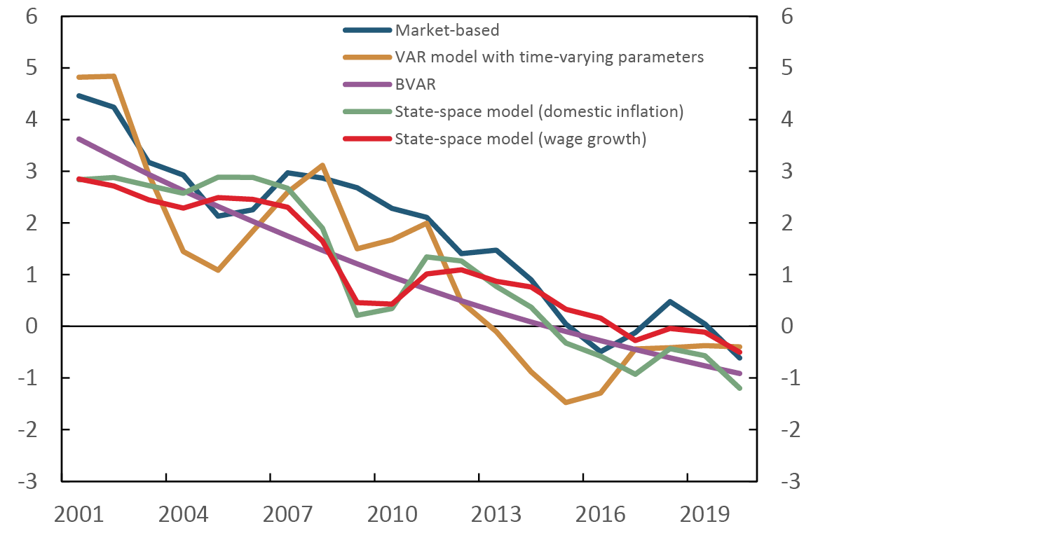
Source: Norges Bank
1 This box is based on Brubakk, Ellingsen and Robstad (2018).
2 For a description of the method, see Lubik and Matthes (2015).
3 The model is inspired by Holston, Laubach and Williams (2017).
4 According to papers published by A.W. Phillips in 1958, a country could choose between low unemployment and low inflation. This choice is often referred to as the Phillips curve.
5 The data used are for the rise in prices for domestically produced goods and services that have historically been higher when correlated with domestic capacity utilisation than aggregate consumer price inflation. We also estimate a version of the model where wage growth is used as the observable variable.
6 We use the so-called Kalman filter (see eg Hamilton (1994)).
7 See Primiceri and Lenza (2020) and Holston et al (2020) for a description of the methods used to adapt the models to the Covid pandemic.
8 See page 51 of Monetary Policy Report 3/16.
3.4 Monetary policy response to shocks
3.4.1 Literature and international practice
In principle, the optimal interest rate response to different types of shocks can be derived if a core model is used that adequately captures the monetary policy transmission mechanism, in both qualitative and quantitative terms, and has a specified loss function (see “Modelling objectives and trade-offs: Loss functions”). An exercise of this type can be a useful guide to how monetary policy should be oriented. In addition, it can serve as an aid to ensuring that a central bank’s response pattern is consistent over time. For these reasons, Norges Bank uses model simulations based on an optimal policy as input to its analyses and projections. The exact interest rate response derived from such simulations is naturally highly model-dependent and should therefore not be taken literally. However, the qualitative results from such optimal policy simulations are usually relatively general, particularly how Norges Bank should respond to demand- and supply-side shocks respectively.
Demand shocks normally pull inflation and output in the same direction, at least in a closed economy, and entail less conflict between the monetary policy objectives. Such shocks should largely be addressed using policy rate changes. A pronounced fall in demand should prompt a marked policy rate reduction that should as far as possible sustain the level of economic activity and contribute to preventing a fall in inflation. Conversely, a positive demand shock should prompt an increase in the policy rate. In a closed economy, demand shocks do not lead to a conflict between objectives and, should, in principle, be neutralised by monetary policy. In an open economy, some conflict will arise owing to the exchange rate channel.85
Supply-side shocks, for instance higher wage growth at a given unemployment rate or changes in price margins in product markets, can to a greater extent give rise to conflict between the inflation target and the objective of high and stable output and employment because supply-side shocks pull inflation and output in opposite directions. In general, economic theory suggests that a shock resulting in higher wage and price inflation should be addressed by a rate increase. Most models indicate that the policy rate increase should be of a magnitude that more than counteracts the isolated fall in the real interest rate (nominal interest rate less expected inflation) that follows from higher inflation prospects, so that the real interest rate rises.86 The magnitude of an interest rate change in response to a supply-side shock, or more generally shocks that lead to a conflict between inflation stability and real economic stability, depends on the central bank’s trade-offs between the objectives.
Uncertainty poses a challenge to monetary policy when it comes to determining the appropriate monetary policy response to different shocks. There are many different types of uncertainty. One way of distinguishing between them is to ascertain whether the uncertainty is quantifiable, often referred to as Knightian uncertainty, named after the US economist Frank Knight (1885–1972), who distinguished between quantifiable risk and uncertainty. Knightian uncertainty is more fundamental and difficult for economic policy to manage. A common strategy to address this type of uncertainty is the minimax principle whereby one seeks to minimise the likelihood of, or cost of, the worst conceivable outcome. The implications of Knightian uncertainty for monetary policy are not entirely unequivocal, but findings generally suggest that central banks should respond more aggressively when facing such uncertainty.87
Quantifiable uncertainty (which Knight called “risk”) is more manageable in principle. A distinction is often drawn between additive and multiplicative uncertainty. Additive uncertainty is not affected by monetary policy. An example of additive uncertainty is uncertainty about future developments in oil prices, global economic cycles, weather conditions and other types of variables that are not influenced by monetary policy. In linear models with additive uncertainty, certainty equivalence applies. That means that the degree of uncertainty should not matter for the monetary policy stance, so that monetary policy can regard projections of uncertain variables as though they were not uncertain.
Linear models are often useful, particularly when there are relatively limited economic fluctuations close to the economy’s long-term equilibrium level. But in some situations it may be important to take non-linearities into account. In that case, certainty equivalence does not apply, even in the case of additive uncertainty. A relevant example is a situation where the policy rate is not far from the effective lower bound. The lower bound for the policy rate is an obvious non-linearity, increasing the risk of the policy rate reaching the lower bound where it is no longer effective as a stabilisation instrument. An intuitive strategy for reducing that risk can be to “keep the ammunition dry” by responding less than otherwise to shocks, leaving some room to respond if a severe negative shock were to arise. Economic theory, on the other hand, suggests that the opposite response is appropriate: one should respond more aggressively to shocks in order to underpin inflation and the activity level.88 This will reduce the likelihood that the lower bound becomes binding and reduce the depth of a downturn.
Multiplicative uncertainty is influenced by monetary policy. Examples of multiplicative uncertainty is uncertainty about the effect of the policy rate on the exchange rate and demand, uncertainty about the slope of the Phillips curve and uncertainty about expectations formation. The monetary policy response pattern can influence this type of uncertainty. A key finding in the literature is that uncertainty about the effect of monetary policy on target variables would suggest a more cautious response to economic shocks,89 because with this type of uncertainty, monetary policy can also contribute to unintended changes in the target variables if the monetary policy effect is not as expected. Responding less (ie more cautiously) to shocks reduces the extent of such unintended changes. This must be weighed against the fact that the achievement of monetary policy objectives improves by responding adequately to shocks if the effect proves to be as expected. Because there will always be a degree of uncertainty about the effects of monetary policy, the precautionary principle will always apply to a certain extent, even if the degree of uncertainty may vary with the economic situation and interest rate level.
A cautious response is often associated with a gradual approach in monetary policy, but cautious is, at least in theory, not exactly the same thing as gradual. A cautious response means that the central bank responds less to a shock than otherwise. A gradual response means that the response to a shock is normal, but that the response comes in a series of smaller increments over time. There may be reasons to change policy rates gradually, but those reasons are not directly related to uncertainty.
A gradual approach can improve the central bank’s ability to affect long-term interest rates and can have a favourable effect on inflation expectations.90 A gradual approach may also be warranted if it increases the central bank’s knowledge about the effects of a change in the policy rate.91 In practice, however, it is not as easy to distinguish between a cautious and a gradual approach, and the distinction is unlikely to be as sharp in policymakers’ judgement-based assessments as it is in theory.
Not all multiplicative uncertainty suggests a more cautious response. If, for example, there is uncertainty about the extent to which inflation expectations depend on previous actual inflation outcomes, theory argues that the response to shocks affecting inflation should be more aggressive.92
Model uncertainty is a type of uncertainty that has elements of both Knightian uncertainty and multiplicative uncertainty but is difficult to specify. Models are always simplifications and build on assumptions with varying degrees of realism. A common response to model uncertainty is to use several different models that build on different assumptions. The model-based predictions can then be taken into account on a discretionary basis. The challenge is that there are no good objective guidelines on how to combine information from different models on a discretionary basis.
Another strategy to address model uncertainty is to use simple rules as a guide to interest rate setting. The Taylor rule is an example of such a simple rule.93 Research shows that certain simple rules for monetary policy, if properly designed, can be relatively robust to model uncertainty.94 Simple rules are commonly used as cross-checks by central banks, even if reference is not always made to the use of such rules in monetary policy reports and the like. The US Federal Reserve is the central bank that most actively uses simple monetary policy rules in its communication.95
3.4.2 Norges Bank’s practice and communication
Norges Bank is one of the few central banks that publishes a policy rate forecast (see Section 3.1 for further details on the policy rate path). When a shock occurs, the Bank will normally respond by changing the policy rate and/or the policy rate path. These instruments are not independent of each other, however, as the rate path represents the forecast for the average policy rate in each quarter. Since Norges Bank usually changes the policy rate stepwise, often by quarter percentage points, the average policy rate will often differ slightly from the level in the policy rate path. The Bank bases its decisions on the assumption that the uncertainty surrounding the rate path is symmetrical, ie if the path is, for example, closer to 1.50% than 1.75%, it is more likely that the policy rate will be 1.50% than 1.75% in the relevant period.
The rate path is derived using the macroeconomic model NEMO, but judgement-based assessments and information from other models also influence the Bank’s policy rate forecasts. There is considerable uncertainty about the policy rate forecast. If the economic outlook, the risk outlook or Norges Bank’s assessment of how the economy functions change, the policy rate will be set at a different level than implied by the rate path.
A single rate path provides little information about the monetary policy response pattern. But a change in the path from one monetary policy report (MPR) to the next reflects the Bank’s reaction to new information since the preceding MPR and any new assessments of economic relationships and the risk outlook.
As a guide to the response pattern for the public and market participants, the Bank publishes a decomposition of the different factors (different shocks) behind the change in the rate path from one MPR to the next. The macroeconomic model NEMO is used as an aid to identify and quantify such shocks, but there is no mechanical relationship between the projections for the shocks and the effects on the policy rate path. Chart 3.4 shows the decomposition in MPR 4/19. The columns show the different factors’ contributions. The black line shows the overall change in the rate path.
Chart 3.4 Factors behind changes in the policy rate forecast between MPR 3/21 and MPR 4/21. Cumulative contribution
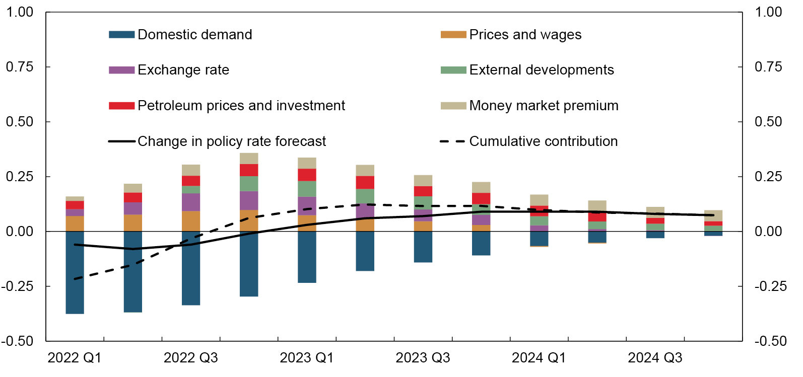
Source: Norges Bank
To some extent, the decomposition provides a fairly detailed description of Norges Bank’s response to different shocks, but it only quantifies the implications of these shocks for the rate path itself. If the Bank’s estimates of the size of the different shocks are known to the public, the decomposition would in principle be a complete description of the response pattern. But the size of the shocks, as estimated and interpreted by Norges Bank, are not communicated in full, partly because there is no unequivocal way of identifying and quantifying shocks. The decomposition must therefore be seen as an aid to help the public and market participants understand the main features of the response pattern and not a complete and detailed description of it. In addition, a complete description of the response pattern is probably nether desirable, nor possible, as it would give the impression of a level of precision that does not reflect the monetary policy assessments in practice. Among inflation-targeting central banks, Norges Bank is probably the central bank that goes farthest in specifying the normal monetary policy response pattern.
The policy rate path can deviate from the market’s policy rate expectations. This does not necessarily mean that Norges Bank’s response pattern is not well understood by market participants. Analyses show that revisions of the market’s interest rate expectations from one publication date to just ahead of the next (the day before), which typically reflect new information between the publication dates, are strongly correlated with revisions of Norges Bank’s policy rate path.96 This indicates that market participants have a good understanding of the Bank’s response pattern and how monetary policy will react to news about economic developments.97 If market participants believe that economic developments will differ from those assumed by the Bank, their policy rate expectations might differ from the rate path, even if the market has perfect knowledge of the Bank’s response pattern.
Analyses nevertheless indicate that publication of the policy rate path influences market expectations in the desired direction. The rate path and the decomposition also reflect the Bank’s assessment of uncertainty and the implications of that uncertainty for the policy rate, as well as the implications for policy rate setting of the risk associated with financial imbalances, as discussed in Section 2.3. The Monetary Policy and Financial Stability Committee’s monetary policy strategy statement describes how the Bank generally takes account of uncertainty: “The policy rate influences inflation and the real economy with a lag, and the effects are uncertain. To reduce the risk of monetary policy contributing to economic instability, Norges Bank will normally respond less forcefully to shocks than if there had not been uncertainty about the transmission of monetary policy. Furthermore, the policy rate is normally changed gradually to make monetary policy more predictable and to reduce the risk of undesirable financial market volatility and unexpected reactions of households and firms.”
In the period following the global financial crisis in 2008, when domestic and international interest rates fell to historically low levels, Norges Bank gave particular weight to caution in policy rate setting. The uncertainty about the effects of policy rate changes is greater than normal in such situations both because there is generally a more limited empirical basis for quantifying the effect of policy rate changes when the rate is at abnormal levels, and in particular because we know little about how policy rate changes pass through to banks’ deposit and lending rates when the policy rate is close to the lower bound. In the Monetary Policy and Financial Stability Committee’s monetary policy strategy statement, reference is also made to situations where a more aggressive response may be appropriate: “In situations where the risk of particularly adverse outcomes is pronounced, or if there is no longer confidence that inflation will remain low and stable, it may be appropriate to react more forcefully than normal in interest rate setting.” This minimax principle was given weight when the policy rate was cut sharply in 2008 in response to the substantial uncertainty during the global financial crisis.
Scenario analysis is one way of describing parts of the response pattern, particularly for situations that are not considered part of normal cyclical fluctuations. On a few occasions, Norges Bank has used scenario analysis as part of its monetary policy strategy and communication. One example is the box in MPR 4/19, which describes potential effects, including monetary policy reactions, of different outcomes of the international trade conflict.98
The Bank uses simple monetary policy rules to some extent as cross-checks in interest rate setting. The role of such cross-checks in the monetary policy decision-making process and in communication has varied somewhat in practice over time. Many of the monetary policy reports have presented different simple rules, showing how the policy rate would have evolved in the near term had those rules been followed. In addition, the market’s interest rate expectations are used as a cross-check for the policy rate forecast. The Bank continuously works on analysing and developing good cross-checks for interest rate setting and projections for inflation and activity levels for use in the decision-making process. The aim is to be as certain as possible that the rules we use as cross-checks are actually robust to model uncertainty, so that they can be given a clearer role in monetary policy assessments and communication.
3.4.3 Monetary policy response to large unusual shocks
Most of the evolution of monetary policy theory and practice has up until recently focused on monetary policy’s role during more or less normal business cycles. But large, unusual shocks sometimes occur that challenge conventional thinking about the role of monetary policy and its instruments. Over the past 15 years, the global economy has been hit by two large, unusual shocks: the global financial crisis of 2008–2009 and the Covid-19 pandemic that broke out in 2020. A characteristic of this type of large, unusual shock is that monetary policy tools are not adequate to bring the level of activity up to a normal level before the shock eventually begins to fade. Monetary policy can be inadequate owing to the size of the shock or its characteristics.
There are two aspects of large, unusual shocks that have implications for the monetary policy strategy. One is that the policy rate can move down to the effective lower bound, where a further cut in the policy rate will not pass through to market rates. The central bank must then consider alternative instruments, described in more detail in Section 3.5 below. The other aspect is that such shocks can necessitate the use of additional measures from other policy areas, in particular fiscal and macroprudential policy.
The global financial crisis showed that price stability does not necessarily lead to financial stability and that international financial markets are so closely integrated that financial market stress in one country can rapidly transmit to the rest of the world. During the global financial crisis, the main challenge was primarily the size of the shock and not its characteristics. The downturn can be regarded as a traditional, negative Keynesian demand shock caused by a financial crisis. The lower bound for the policy rate prevented monetary policy in many countries from becoming sufficiently expansionary to counteract the shock. Many central banks therefore used alternative instruments (see Section 3.5).
The Covid-19 pandemic was both a large and an unusual shock. Widespread business closures and mobility restrictions led to a sharp fall in the level of activity. At the same time, this was in a sense a desirable fall as it was considered necessary for Covid-related purposes. The business closures and mobility restrictions represented in isolation a negative supply shock. At the same time, the drop in output, and thereby income, also had negative consequences for demand. In an influential article, Guerrieri et al. (2020) introduce the term “Keynesian supply shock” about the type of shock the pandemic represented. Their point is that the negative supply shock created a fall in demand that was greater than the initial fall in supply. The net effect was therefore deficit demand in the Keynesian sense, at the same time as supply was limited. In contrast to traditional negative supply shocks, where a tighter economic policy is needed to bring aggregate demand down to match lower potential output, a Keynesian supply shock requires an economic policy that is more expansionary.
Another distinguishing feature of the pandemic was that monetary policy was far from adequate to counteract its effects. This was to some extent because the lower bound for the policy rate restricted monetary policy, as it did during the global financial crisis, but primarily because Covid-related restrictions created a need for measures targeting those more directly hit by the restrictions. Fiscal support measures and redistribution are primarily a fiscal policy responsibility, and fiscal measures were used on a large scale both in Norway and in other countries. In Norway, monetary policy’s most important role at the beginning of the pandemic was to ensure well-functioning credit markets and lower borrowing costs for enterprises and households. Even though economic activity was severely reduced as a result of Covid-related restrictions, the policy rate cuts supported activity in those segments of the economy that were not directly hit by the restrictions. Expansionary monetary policy, for example, contributed to a high level of housing investment, which offset some of the fall in the level of activity in those segments of the economy that had been closed down. Nevertheless, fiscal policy and its direct support measures must be said to have been the most important policy instrument during the pandemic. The interactions between monetary policy and fiscal policy are described in more detail in Section 3.6.
85 See Røisland and Sveen (2018).
86 Called the Taylor principle.
87 Gerke, Hammermann and Lewis (2009).
88 See Reifschneider and Williams (2000).
89 This is commonly referred to as the Brainard principle. See article by Brainard (1967).
90 See Goodfriend (1991) and Woodford (2003).
91 See Sack (1998).
92 See Söderström (2002).
93 See Taylor (1993).
94 See Taylor and Williams (2011).
95 See the Monetary Policy Report to the Congress, page 36, and the Cleveland Fed’s 7 simple monetary policy rules (which are also used to forecast the policy rate).
96 See Brubakk, ter Ellen and Xu (2017).
97 Households also seem to understand the Bank's response pattern, see Erlandsen and Langbraaten (2018) (https://bankplassen.norges-bank.no/2018/12/20/far-folk-med-seg-norges-banks-signaler-om-renten/)
98 It was emphasised that these monetary policy reactions are based on model simulations in the core model NEMO and are therefore not based on an assessment by decision makers of what an appropriate monetary policy response in the different scenarios would be.
3.5 Alternative instruments
The economy may, at times, be subjected to such large negative shocks that the policy rate cannot be set as low as the shock might warrant because there is a limit to how low the policy rate can be set and still pass through to banks’ lending and deposit rates. At the same time, the effect of negative interest rates on parts of the financial market may be uncertain. As an alternative to further reducing the policy rate, the central bank can utilise other instruments.
After the GFC in 2008, monetary policy was stretched far by many of our trading partners, and even further in a number of countries in connection with the Covid pandemic. Some have lowered their policy rates to below zero. A number of central banks have also used their balance sheet to underpin economic activity and inflation.
3.5.1 International experience
Other central banks have used their balance sheet in different ways to stimulate demand. The most common measures have been asset purchases, mainly government bonds, and extraordinary loans to banks.
The purpose of central bank purchases of bonds is to push down long-term interest rates. The purchases push up prices, and push down effective yields, on the bonds purchased. To the extent that the bond sellers shift demand towards other securities, for example equities, those prices may also increase. Central banks’ securities purchases can also have an impact by signalling continued low policy rates.
Extraordinary loans to banks have been used to support credit growth by giving banks lower and more predictable funding costs. Such loans feature special terms and normally have substantially longer maturities than loans provided to manage liquidity in the banking system in a normal situation. Many central banks have provided extraordinary loans with interest rate terms linked to whether banks sustain or boost growth in credit to households and enterprises.
The central banks of Switzerland and the Czech Republic have taken direct action in the foreign exchange market. Both central banks set an upper limit on the value of their currencies against the euro and signalled that they would sell as much of their own currency against the euro as necessary to achieve that. The aim was to underpin inflation to keep it closer to target than would otherwise have been the case. Both countries maintained their currency floor for more than three years.
Several studies indicate that alternative instruments in other countries have had an impact on interest rates and financial prices. The measures also appear to have stimulated activity, supported banks’ credit provision and underpinned inflation expectations. But it is difficult to precisely estimate the magnitude and duration of the effects. The choice of method and assumptions influences the results, and the estimates tend to vary. Studies also suggest that alternative instruments have the strongest effect in a situation with market imbalances and high risk premiums. As interest rates and risk premiums decline, or when the policy rate nears its lower bound, the effect appears to have weakened.
3.5.2 Alternative instruments in Norway
During both the GFC in 2008 and in connection with the pandemic in spring 2020, Norges Bank implemented extraordinary measures to mitigate market volatility and avoid destabilising effects on the economy. During both crises, lending to banks was substantially higher than normal. Loans with longer maturities and loans in USD were also provided. The list of securities eligible as collateral for loans from Norges Bank was also expanded. During the GFC, Norges Bank administered a swap arrangement on behalf of the government, where banks could temporarily swap covered bonds against short-term government securities. During the crisis in March 2020, Norges Bank communicated that intervening in the foreign exchange market could be appropriate for maintaining a well-functioning NOK market, and a limited amount of NOK was subsequently purchased.
Negative policy rate
The policy rate is the normal monetary policy instrument. Evidence suggests that a downturn in the Norwegian economy should initially be addressed by lowering the policy rate. In May 2020 the policy rate was reduced to zero percent. This reduction passed through to money market rates and, to a great extent, also to banks’ lending rates. Central banks in a number of other countries have set their policy rates below zero. Negative policy rates have systematically passed through to money market rates. This is because cash is a costly alternative to electronic money in the money market. In Norway, most borrowing is at a floating rate which means that most of banks’ funding is also at floating rates. Lower money market rates are therefore rapidly reflected in banks’ wholesale funding rates. The transmission to interest rates facing the general public may weaken, however, when the policy rate approaches zero and turns negative. This is because banks are reluctant to set negative rates on deposits that customers can withdraw and keep as cash at little cost. This means that the effect of a policy rate cut on banks’ funding costs fades when the policy rate is reduced to below zero. In isolation, this suggests that the transmission from the policy rate to interest rates facing the general public is likely weaker in that case than when the policy rate is reduced from higher levels. At the same time, evidence suggests that the effect of a policy rate cut on the exchange rate is sustained when the policy rate is negative. However, the effect of a negative policy rate on the financial markets is uncertain, and there is a risk that undesirable and unintended effects may occur.
Extraordinary loans to banks
Norges Bank provides loans to banks on a regular basis in connection with the implementation of monetary policy. The purpose of the loans is to manage overall liquidity in the banking system so that the shortest money market rates are kept close to the policy rate. The purpose of extraordinary loans, on the other hand, is to make monetary policy more expansionary by stimulating credit growth and economic activity.
Long-term loans to banks, with or without credit growth requirements, will likely be most effective in a situation where premiums in banks’ funding markets are high or banks face funding problems. The instrument works by lowering funding costs for banks and can contribute to facilitating household and corporate access to credit.
A situation may also arise where it may be appropriate to provide loans in order to bring Nibor rates down towards the policy rate. This may be the case if the policy rate is low and further cuts are not deemed appropriate, at the same time as Nibor is markedly higher owing to high risk premiums.
Extraordinary loans to banks will add more reserves to the banking system than the sum of banks’ quotas in Norges Bank’s liquidity management system. To prevent the shortest money market rates from falling below the policy rate, (i) the extra liquidity supplied must be withdrawn by providing F-deposits, the reserve rate must be raised and set equal to the policy rate or (iii) the quotas must be increased so that all deposits bear interest within the quota. During the Covid pandemic, extraordinary loans were provided to banks with terms of up to one year. Norges Bank announced in advance that the extra liquidity supplied would be withdrawn using intraday F-deposits. This gave banks daily access to the extra liquidity, while maintaining the quota system for liquidity management (see box on liquidity management in Norway).
As in the case of Norges Bank’s ordinary loans to banks, extraordinary loans can only be provided against eligible collateral. The value of the collateral, after a risk haircut, determines the size of the lending facility. If large loans are needed, the volume of eligible collateral can constitute a limitation of the size. In such a situation, the Bank must determine whether the range of eligible collateral should be expanded, and whether it is in keeping with statutory requirements for adequate loan collateral.
Purchases of securities
For borrowers with floating-rate loans, long-term interest rates are relevant primarily as a signal of short-term interest rate expectations. In countries with a higher proportion of fixed-rate loans, changes in long-term interest rates can have a more direct effect on credit demand and disposable income.
The Norwegian bond market is small, with foreign investors accounting for a large share of bondholders. Although Norwegian government securities have the highest rating, rates can vary fairly widely in relation to other Norwegian rates, partly owing to variations in liquidity premiums over time. It is uncertain whether lower long-term government bond yields would have had a broad impact on interest rates facing households and enterprises. An effect via lower expected policy rates would probably have had an impact, but it is more uncertain whether lower term premiums on Norwegian government bonds would impact other interest rates. Purchases of government securities can result in a weaker krone if foreign investors divest their positions, but the magnitude of such an effect is difficult to predict.
Measured in terms of volume outstanding, covered bonds constitute a bigger market than government securities in Norway. Most NOK-denominated covered bonds are issued with a floating rate. Banks own a large share as part of their liquidity portfolios. In other countries, central banks have purchased covered bonds when risk premiums have been high. In Norway, covered bonds were used in the swap arrangement offered from November 2008 to October 2009. Covered bond purchases or swaps can be seen as an alternative to long-term loans to banks.
Exchange rate measures
For small open economies like Norway, the exchange rate is an important monetary policy channel. In a situation where low inflation prospects threaten confidence in the inflation target and further policy rate cuts are not deemed appropriate, exchange rate measures can be effective. Both Switzerland and the Czech Republic set a floor for the value of their currencies against the euro. Both are inflation-targeting countries. Such a measure increases the risk exposure of the central bank’s equity capital. As long as the exchange rate floor is in operation, foreign exchange market conditions will determine how much foreign exchange the central bank has to buy. The size of the central bank’s balance sheet is thus determined by market developments. If the country’s currency appreciates when the measure is withdrawn, there is a risk that the central bank loses all or part of its equity capital as it is measured in domestic currency. However, in principle, a central bank can operate with low or negative equity capital, although this may undermine confidence in the central bank and in nominal stability.99
Norges Bank’s assessments
A set of overriding principles underpins Norges Bank’s use of instruments. Norges Bank must by law require adequate collateral for credit. Adequate collateral is defined in principle as the securities approved in Norges Bank’s system for collateral and related haircut rates. Any measures that entail credit risk materially beyond this should in principle be approved by the political authorities and be recognised in the central government’s balance sheet, even if Norges Bank is responsible for operational implementation. Furthermore, any extraordinary measures should be designed to be as neutral as possible, ie the measures are targeted at well-defined groups of counterparties rather than at individual institutions, so that counterparty institutions can participate on equal terms. As a main rule, auctions should be used when implementing extraordinary measures.
Norges Bank will normally be very reluctant to set a negative policy rate, partly because it may have an undesirable and unintended impact on financial markets. However, the Bank does not rule out that it could become relevant, for example, if there is a need for a very expansionary monetary policy stance in a situation where financial market stress results in tight financial conditions despite other measures such as extraordinary loans to banks.
It is less relevant for Norges Bank to use instruments such as government bond purchases to influence long-term rates because the share of fixed-rate loans is relatively low and Norway’s government bond market is much smaller than in many other countries. The Bank’s assessment is that the costs of using such instruments may outweigh the benefits. Norges Bank would have to be faced with exceptional circumstances to use foreign exchange market interventions to increase the degree of monetary accommodation in situations where the room for further policy rate reductions has been exhausted. However, in response to extraordinary conditions in the NOK market, interventions could be warranted to help stabilise the market, as the Bank did in March 2020.
In Norway, alternative monetary policy instruments appear most appropriate in situations with substantial market turbulence or if a risk of deflation were to arise. An important reason why Norges Bank is more reluctant to use of alternative instruments is that there is substantial room for manoeuvre in fiscal policy in Norway and a tradition for fiscal policy to contribute to stabilisation policy. (See Section 3.6 for a detailed discussion of the interaction between monetary and fiscal policy.)
99 See Chapter 13 of “Ny sentralbanklov. Organisering av Norges Bank og Statens pensjonsfond utland”, Official Norwegian Reports (NOU) 2017, for a further discussion (in Norwegian only).
3.6 Interaction between monetary policy and fiscal policy
In general, there are arguments in favour of using both monetary and fiscal policy to stabilise the economy. The Tinbergen principle states that there must be a tool for each policy goal if all the goals are to be achieved. With two tools – monetary and fiscal policy – two goals can be achieved, at least if the tools are coordinated, for example price stability and real economic stability.
There are, however, some institutional challenges associated with coordinating monetary and fiscal policy, primarily with regard to central bank independence. Granting independence to central banks was a way to bring soaring inflation in the 1970s and 1980s under control. By shielding policy rate decisions from the political sphere, it was easier to achieve a sufficiently contractionary monetary policy to bring down inflation. International experience, supported by extensive political economy research, shows that there is a risk of expansionary bias when politicians decide on economic policy because short-term considerations, such as high economic growth, may be prioritised ahead of long-term considerations in order to win votes. This bias can lead to high inflation and excessive public debt. While central bank independence and explicit mandates about price stability solved the first problem, fiscal rules were a means to prevent bias in the form of excessive budget deficits. Because such rules, which restricted government spending, also entailed limitations on the extent to which fiscal policy could be used to stabilise the economy (apart from via automatic stabilisers), central banks came to play the main role in cyclical policy, to the extent this did not conflict with price stability objectives.
In Norway, fiscal policy has historically had a somewhat larger role in stabilisation policy than in many other countries. Before inflation targeting was introduced in Norway, fiscal policy was the main stabilisation tool. The introduction of an inflation target for monetary policy in 2001 gave monetary policy a larger role in stabilisation policy. The regulation issued in 2001 states that monetary policy shall underpin fiscal policy by contributing to stable developments in output and employment. But fairly soon after the regulation had been issued, the description of the division of labour between monetary policy and fiscal policy changed and was replaced by formulations that monetary policy is the “first line of defence” in stabilisation policy.
A fiscal rule for the spending of petroleum revenues was introduced at the same time as inflation targeting was formalised. Norway’s fiscal rule is only based on cross-party consensus and has no legal foundation. The rule was introduced to ensure a gradual phasing-in of oil revenues while providing room for flexibility by allowing for temporary deviations from the rule based on cyclical considerations. Even though monetary policy has been the first line of defence, fiscal policy has also had a role in smoothing the business cycle, both in the form of traditional automatic stabilisers within the fiscal rule and in the form of discretionary deviations from the rule to stabilise the economy.
There has been little or no coordination of monetary-fiscal policy interactions. Interaction since 2001 can perhaps be most accurately described as a kind of Stackelberg equilibrium where fiscal policy is the leader and the central bank is the follower and where fiscal policy setting has internalised the central bank’s response pattern.100 The policy mix produced by the Stackelberg equilibrium is generally not as good as that resulting from policy coordination, but can be better than a Nash equilibrium, where the policy areas seek to achieve their respective goals independently of each other.
The view of the division of roles between monetary policy and fiscal policy has been characterised by the type of shocks thought to be the most important. With a pure demand shock, there is no conflict between price stability and real economic stability, at least in a closed economy, and in principle only one instrument is required. Fiscal policy will then only have a role if the room for manoeuvre in monetary policy has been exhausted and further stimulus is needed.
When inflation targeting was introduced, the business cycle was expected to be driven by demand shocks to a greater extent than subsequently proved to be the case. With supply shocks (such as China’s strong export growth through the 2000s), monetary policy alone could not achieve the inflation target and fulfil the objective of stability in the real economy at the same time. In an open economy, where the exchange rate affects imported price inflation, there will also be some degree of conflict between the two objectives during demand shocks. Experience of inflation targeting has shown that the central bank must as a rule make a trade-off between different objectives and considerations in the short term.101
The Covid-19 pandemic has changed the way economists internationally think around the role of fiscal policy. While the primary emphasis used to be on ensuring the sustainability of public finances through rules-based fiscal policy, there is now greater focus on the role of fiscal policy as a stabilisation tool and not least on the allocation of risk via transfers and redistribution when large shocks impact different groups in different ways, as when businesses closed down during the pandemic. Experience showed that in the face of extreme shocks, such as the pandemic, neither monetary policy nor fiscal policy alone can shield the economy from a severe downturn. The need for an appropriate monetary-fiscal policy interaction was the theme of the Geneva report in 2021102 and was also one of the topics researched by the ECB in preparing its strategy review103.
The National Budget for 2022104 notes that fiscal policy was able to very quickly provide income support to households and enterprises hard hit by Covid-related restrictions through direct transfers and liquidity support. The policy rate, on the other hand, is a blunt instrument and cannot be used to target individual sectors in the same way. According to the National Budget, it is therefore important that in crisis situations the two policy areas are considered together. Fiscal policy will also be important in situations where a downturn is having a broad impact on the economy, but where the room for further policy rate cuts has been exhausted.
How far different countries will go in implementing closer monetary-fiscal policy interaction is so far unclear. Even though the pandemic has shown that some situations require the active use of both monetary and fiscal policy instruments, close interaction also presents challenges. Some have voiced concern that the central bank’s independence might be threatened. A related concern is that owing to the high level of public debt in many countries, which increased further as a result of the pandemic, there is a risk of fiscal dominance, which is a situation where the central bank cannot or will not raise the policy rate to stabilise inflation because this will further exacerbate the government’s debt situation. As a result, the level of inflation is in practice determined by fiscal policy and not monetary policy. In Norway, however, there is little risk of fiscal dominance as the government is in a net asset position because of the oil revenues saved in the Government Pension Fund Global.
Even though there are reasons for monetary policy and fiscal policy not to be coordinated, in the sense that that the two instruments are wielded in tandem, there are good reasons for adequate information sharing between the policy areas. This was also pointed out in the National Budget for 2022, in which the Government writes that “[i]t is particularly important that fiscal policy and monetary policy are formulated based on a common understanding of the economic situation and the effects of these policies, both individually and in concert”.
100 For an analysis of such interaction between monetary and fiscal policy, see Steigum (2000). Samspillet mellom pengepolitikken og finanspolitikken ved et inflasjonsmål (Norwegian only).
104 Meld. St. 1 (2021–2022) – regjeringen.no (in Norwegian only). Information in English: The National Budget 2022 – regjeringen.no
Literature
Aastveit, K.A., K.R. Gerdrup and A.S. Jore (2011) “Short-term forecasting of GDP and inflation in real-time: Norges Bank’s system for averaging models”. Staff Memo 9/2011. Norges Bank.
Alsterlind, J., M. Lindskog and T. von Brömsen (2020) “An index for financial conditions in Sweden”. Staff Memo February, Sveriges Riksbank.
Bernhardsen, T. and K. Gerdrup (2006) “Den nøytrale realrenten”. Penger og Kreditt 4/2006. Norges Bank (in Norwegian only).
Brainard, L. (2018) What Do We Mean by Neutral and What Role Does It Play in Monetary Policy? Tale. Detroit Economic Club, Michigan. 12 September.
Brainard, W. (1967) “Uncertainty and the Effectiveness of Policy”. American Economic Review, 57(2), pp 411–425.
Brander A., H. Brekke, B.E. Naug and F. Eger (2017) “Evaluering av Regionalt nettverk” [Evaluating the Regional Network]. Staff Memo 3/2017. Norges Bank.
Brouillette,S., G. Faucher, M. Kuncl, A. McWhirter and Y. Park (2021) “Potential output and the neutral rate in Canada: 2021 Update”. Staff Analytical Note 2021-16, Bank of Canada.
Brubakk, L., J. Ellingsen and Ø. Robstad (2018). “Estimates of the neutral rate of interest in Norway”. Staff Memo 7/2018. Norges Bank.
Brubakk, L., S. ter Ellen and H. Xu (2017) “Forward guidance through interest rate projections: does it work?”. Working Paper 6/2017. Norges Bank.
Canova, F., F. Furlanetto, F. Smets and V. Wieland (2019) “Review of macro modelling for policy purposes at Norges Bank”. Occasional Papers 55/2019. Norges Bank.
Gerdrup, K.R., E.M. Kravik, K.S. Paulsen and Ø. Robstad (2017) “Documentation of NEMO – Norges Bank’s core model for monetary policy analysis and forecasting”. Staff Memo 8/2017. Norges Bank.
Gerdrup, K.R. and R.N. Torstensen (2018) “The effect of higher interest rates on household disposable income and consumption – a static analysis of the cash-flow channel ”. Staff Memo 3/2018. Norges Bank.
Gerke, R., F. Hammermann and V. Lewis (2009) “More or less aggressive? Robust monetary policy in a New Keynesian model with financial distress”, Discussion Paper Series 1: Economic Studies 2009, 23, Deutsche Bundesbank.
Goodfriend, M. (1991) Interest rates and the conduct of monetary policy. Carnegie-Rochester Conference Series on Public Policy, Vol. 32, pp 7–30.
Guerrieri, V., G. Lorenzoni, L. Straub og I. (2022) “Macroeconomic implications of Covid-19: Can negative supply shocks cause demand shortages?”. NBER Working Paper No. 26918
Hamilton, J.D. (1994). Time Series Analysis. Princeton University Press.
Hesse, H., B. Hofmann and J. Weber (2017) “The Macroeconomic Effects of Asset Purchases Revisited”. BIS Working Papers No 680.
Holston, K., T. Laubach and J.C. Williams (2017) “Measuring the natural rate of interest: International trends and determinants”. Journal of International Economics, 108, January, pp 59–75.
Issing, O. (2019) The Long Journey of Central Bank Communication. Cambridge MA: MIT Press.
Jensen, J.R. and J. Pedersen (2019) “Macro financial linkages in a SVAR model with application to Denmark”. Working Paper No. 134, January, Danmarks Nationalbank.
Kravik, E. and Y. Mimir (2019) “Navigating with Nemo”. Staff Memo 5/2019. Norges Bank.
Lane, P.R. (2019) Determinants of the real interest rate. Speech. National Treasury Management Agency, Dublin. 28 November.
Laubach, T. and J.C. Williams (2003) “Measuring the Natural Rate of Interest”. Review of Economics and Statistics 85 (4), November, pp 1063–70.
Lubik, T.A. and C. Matthes (2015) “Calculating the natural rate of interest: A comparison of two alternative approaches”. Richmond Fed Economic Brief October 2015. Federal Reserve Bank of Richmond.
Norges Bank (2021) “Norges Bank’s liquidity policy: principles and design”. Norges Bank Papers 3/2021.
Reifschneider, D. and J. Williams (2000) “Three lessons for Monetary Policy in a Low-Inflation era”. Journal of Money, Credit and Banking, 32 (4).
Røisland, Ø. and T. Sveen (2018) “Monetary policy under inflation targeting”. Occasional Papers 53/2018. Norges Bank.
Sack, B. (1998) “Uncertainty, Learning, and Gradual Monetary Policy”. Finance and Economics Discussion Series (FEDS) no. 1998-34, Board of Governors of the Federal Reserve System.]
Söderström, U. (2002) “Monetary Policy with Uncertain Parameters”. The Scandinavian Journal of Economics, Vol. 104, No. 1, pp 125–145.
Taylor, J.B. (1993) “Discretion versus policy rules in practice”. Carnegie-Rochester Conference Series on Public Policy 39, pp 195–214.
Taylor, J.B. and J.C. Williams (2011) “Simple and Robust Rules for Monetary Policy”. In: Benjamin M. Friedman and Michael Woodford. Eds. Handbook of Monetary Economics. Vol. 3B, North Holland, pp 829–860.
Vonen, N.H. (2011) “A financial conditions index for Norway”. Staff Memo 7/2011. Norges Bank.
Wicksell, K. (1898) Interest and Prices. London: Macmillan (translated by R.F. Kahn in 1936).
Woodford, M. (2003) Interest and Prices: Foundations of a Theory of Monetary Policy. Princeton University Press.