Expecting the unexpected – can we predict risks to Norwegian GDP-growth?
Deep recessions are damaging for the economy and society as a whole. Having a view on risks to GDP-growth can be crucial for deploying the right policy tools at the right time. I assess if measures of financial imbalances can help quantify risks to GDP-growth in Norway. The results from simple quantile regression analyses are promising.
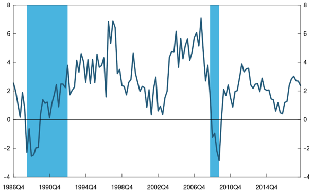
Forecasting recessions is inherently difficult. Norway has since the early 1980s experienced several downturns, but the severe ones have occurred against the backdrop of financial crises, either originating in Norway (late 1980s/early 1990s) or financial stress imported from global markets (2008-09), see Figure 1. Even though it is difficult to predict such events, work done by researchers at the IMF and Federal Reserve Bank of New York, using quantile regressions¹, find that quantifying risks to GDP-growth may be within reach. I apply this method to Norwegian data.
| Figure 1. GDP Mainland-Norway. Financial crisis and stress highlighted in blue. Four-quarter growth |
Standard regression analysis focuses on the mean of the distribution of what we are interested in. The quantile regression technique provides a direct forecast of the different parts of the probability distribution. I will focus on downside risk to GDP-growth, setting this to GDP-growth in the lower 5th percentile. This number will vary over time depending on financial conditions. Loosely speaking we can say that five percent of the time, GDP-growth will be lower than this (time-varying) number.
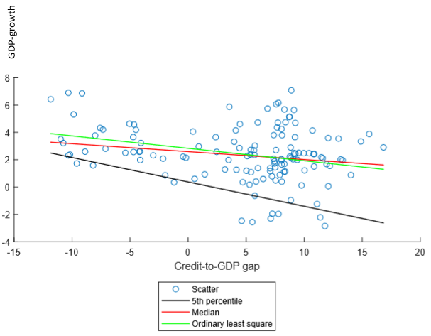
Can indicators of financial imbalances help us quantify the risk to GDP-growth? Figure 2 shows the main results from a quantile regression where I condition on the credit-to-GDP gap. Lagged GDP is also included in the regression. The credit-to-GDP gap is already being used in Norges Bank’s assessment of the countercyclical capital buffer. This indicator (as well as three other indicators used in this blog), are reported on the Bank’s webpage. The regression is set up to forecast GDP-growth three years down the road. The dots in the figure are observations, i.e. the credit-to-GDP gap and GDP-growth for any point in time. The two lines in the middle show the quantile regression line for the median and the ordinary least square regression line for the mean (OLS). The lower line shows the quantile regression line for the 5th percentile. Based on this figure, we should expect that GDP-growth is reduced three years ahead when current credit-to-GDP gap is increasing since the lines in the middle are downward-sloping. More interestingly, the 5th percentile is reduced even more. An implication is that policymakers should consider guarding against a bad economic outcome when measures of financial imbalances are increasing.
| Figure 2. Scatter plot and quantile regression results |
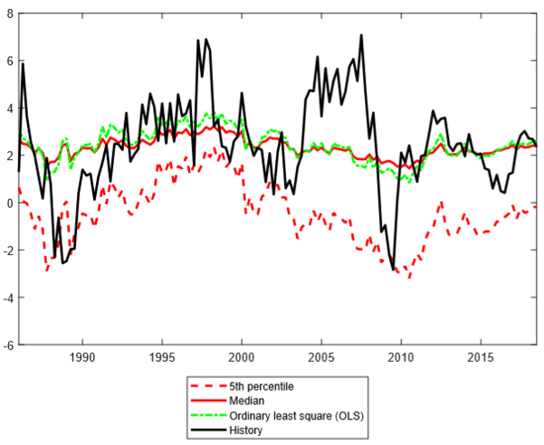
The forecasts from the model are shown in Figure 3. The most likely scenarios are captured in the median and mean (OLS) forecasts. Forecasts for GDP-growth are gradually revised downwards from the late 1990s as the credit-to-GDP gap is increasing in this period, even though the Norwegian economy is booming most of this time. So what happens to downside risks? The figure shows that while growth expectations are reduced somewhat, negative risks to GDP-growth increase markedly. The forecast for GDP-growth in the 5th percentile is reduced from around 0 per cent in 2000 to -2 per cent in early 2009. This means that the model predicts that the severity of a downturn is getting worse year by year, leading up to and including the global financial crisis.
| Figure 3. Quantile regression forecast for GDP using credit-to-GDP as an explanatory variable. Four-quarter growth |
The result from the quantile regression is so far promising. However, a weakness is that the forecast is “in-the-sample”, i.e. we look at the fit in a period included in the estimation. When we do actual forecasts we need to relay on “out-of-sample” exercises, i.e. we must forecast based on a model estimated on historical data. To test for this, I estimate the model on data up to 2006Q1 and assess how successful the model is in predicting GDP-growth in 2009Q1, a quarter with a big drop in economic activity. The first chart in Figure 4 shows the results based on the credit-to-GDP gap. The forecast spans the whole distribution for possible outcomes of GDP-growth. The 5th percentile is highlighted in blue.
Now we know that a financial crisis struck the world economy in 2008, and it is reasonable to assume that Norwegian GDP-growth should be low in the beginning of 2009. As expected, actual GDP-growth in this quarter turned out to be much lower than the central tendency in the model forecast (median shown in red and mean shown in green). However, it was close to the 5th percentile that was forecasted three years in advance. While the actual outcome was bad, the model shows us that the outcome was reasonable, given the history of the credit-to-GDP gap.
| Figure 4. Density forecast for GDP-growth in 2009Q1 based on information up to 2006Q1 using four different financial indicators in the quantile regression |
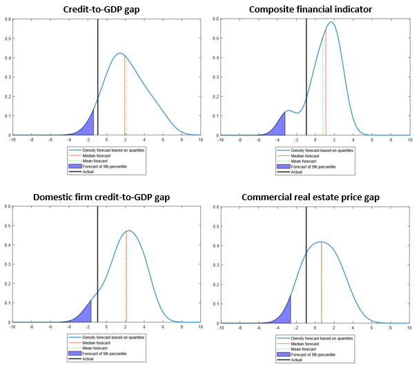
Other indicators could have done an equally good, or better job. For comparison, Figure 4 also shows the density forecasts using other financial variables in the regression. The model forecasts based on the composite financial indicator² and domestic firm credit-to-GDP gap both show signs of downside risks to GDP-growth building up already in early 2006. As a consequence, the mean forecasts are lower than the median forecasts. The last financial indicator in the figure is commercial real estate prices. These prices were high prior to the financial crisis, possibly indicating a high level of financial imbalances and future negative risks to GDP-growth. For this model, both the mean and median forecasts as well as the forecast for the 5th percentile are low.
To summarize, I find that simple quantile regressions based on financial indicators can be used to quantify downside risk to GDP-growth in Norway. These type of models enable us to forecast the size of bad, but not unlikely, outcomes, when measures of financial imbalances are increasing. The conclusions drawn can provide fruitful insights for policymakers.
1 See for example “The Term Structure of Growth-at-Risk”.
2 The variable represent a non-linear transformation of, e.g., house prices, credit to households, credit to non-financial enterprises and bank leverage, which are used to estimate the probability of a financial crisis. This composite variable is probably by construction better at capturing severe risks to GDP-growth (see “Bubbles and Crises: The Role of House Prices and Credit” for more information). However, it suffers here from the drawback of being estimated over the whole sample (also on data after 2006Q1) which means that it may be too good at forecasting the risks to GDP-growth in this case. On the other side, it uses data for many countries and could therefore be more robust. The crisis probability model is also reported on the Bank’s webpage.

0 Kommentarer
Kommentarfeltet er stengt