
FSR 2025 H2
In a nutshell
Continued heightened risk of weakened financial stability
The Norwegian financial system is resilient. At the same, the outlook for the global economy is highly uncertain, in particular due to geopolitical tensions and changes in global trade policy. In a global, interconnected financial system, new shocks may quickly impact the Norwegian financial system.
Lower household debt-to-income ratios
Norwegian households are highly indebted, but debt growth has been slower than income growth in recent years. Debt-to-income (DTI) ratios have declined the most for households with the highest level of debt. This contributed to somewhat lower household sector vulnerabilities.
In the years following the pandemic, high inflation and higher interest rates have led to tighter finances for many households, but most households have been able to service debt and cover normal living expenses with current earnings. Many households also have accumulated savings.
Over the past two years, wage growth has outpaced inflation, and residential mortgage rates have edged down slightly in 2025. This has strengthened household purchasing power and improved debt-servicing capacity.
Developments in commercial real estate are stable but still a challenge for real estate developers
Banks have substantial commercial real estate (CRE) exposures. Higher interest rates and lower property values have posed a challenge for CRE firms, but high employment and increased rental income have enabled most firms to cover expenses with current earnings, while for real estate developers, this is still a challenge. Housing construction is low, and earnings have fallen. Somewhat lower interest rates and higher house prices may boost profitability ahead, but Norges Bank still expects somewhat higher bank losses on loans to real estate developers.
Banks are resilient
Resilient banks are important for financial stability. Norwegian banks are solid, have ample liquidity and low losses. Firms and households have ample access to credit. Maintaining financial system resilience is important. The countercyclical capital buffer requirement makes a contribution in this regard.
The Committee’s assessment
Norges Bank’s Monetary Policy and Financial Stability Committee considers the Norwegian financial system to be robust. Households and firms have solid debt-servicing capacity. Debt-to-income (DTI) ratios have declined over time across households, and vulnerabilities associated with high indebtedness have been reduced somewhat. At the same time, there is still a heightened risk of events that could weaken financial stability. It is important to maintain the resilience of the financial system so that vulnerabilities do not amplify an economic downturn.
Continued heightened risk of events that could weaken financial stability
The balance of risks for the global economy is marked by geopolitical tensions and changes in global trade policy. The effects of higher tariffs remain uncertain. They will likely dampen global growth, but so far do not appear to have significantly affected economic activity, neither in Norway nor among Norway’s main trading partners. At the same time, the framework for international cooperation appears to be more unpredictable than before.
The outlook for the global economy is highly uncertain, and the risk of unexpected events that could weaken financial stability is still higher than normal. Major equity indices have reached new peak levels, and the IMF points out that financial asset valuations appear stretched, increasing the risk of abrupt and disorderly market movements. At the same time, the interconnectedness between banks and other financial institutions is increasing, which could amplify market movements and contribute to stress spillovers in the financial system.
Changes in the security policy landscape have resulted in many European countries now increasing defence investment. At the same time, expenses related to climate transition and an ageing population are rising. Budget adjustments will be particularly difficult in countries with weak government finances and already high government debt. In a turbulent world, the risk of targeted cyberattacks and other operational disruptions also increases. If cyberattacks impact critical functions or cause a broad-based loss of confidence, they could pose a threat to financial stability.
The cryptoasset market is also growing rapidly, particularly stablecoins. Stablecoins are designed to maintain a stable value relative to reference assets, such as the US dollar, and are often backed by reserves in the form of bank deposits and liquid securities. However, if confidence is lost, stablecoins may face a redemption run. Rapid sales of underlying assets can trigger liquidity stress that can spill over to other markets. Should strong stablecoin growth persist, stablecoins may become a source of systemic risk in the global financial system. The new Markets in Crypto-Aassets Regulation (MiCA) contributes to reducing systemic risk. Globally, however, there is still a need for further regulatory developments and cooperation.
In a global, interconnected financial system, new shocks may quickly impact the Norwegian financial system. Financial system vulnerabilities could amplify a downturn in the Norwegian economy and lead to bank losses.
Lower household debt-to-income ratios
The high indebtedness of many households is a key financial system vulnerability as it increases the risk of sharp consumption cutbacks should interest rates rise, household income decline or house prices fall markedly. Should such multiple shocks coincide, consumption cutbacks could weaken firms’ earnings and debt-servicing capacity. Analyses in this Report show that households with the highest DTI ratios cut back on consumption more than other households when interest rates rise and house prices fall markedly.
According to Finanstilsynet’s (Financial Supervisory Authority of Norway) residential mortgage lending survey for 2025, DTI ratios increase somewhat with new mortgages, and a higher share of new mortgages are issued with loan-to-value (LTV) ratios close to 90%. Developments must be viewed in the light of the increase in the Lending Regulations’ maximum LTV ratio requirement at the turn of the year from 85% to 90%. At the same time, total household debt has risen less than income in recent years, and analyses in this Report show that DTI ratios have declined broadly across households and the most for those with the highest ratios. In Norges Bank’s assessment, Norwegian household vulnerability related to high debt has been somewhat reduced. This vulnerability may increase again if looser financial conditions result in rapidly rising house prices and debt.
Higher interest rates and high inflation tightened household finances in the years following the pandemic. However, most households have been able to service debt and cover normal living expenses with current earnings by a solid margin. Many households also have financial buffers. Over the past two years, wage growth has outpaced inflation, and residential mortgage rates have edged down slightly in 2025. This has strengthened household purchasing power and improved debt-servicing capacity.
For a long time, house prices rose faster than household income. At the same time, the owner-occupancy rate has remained firm, Nevertheless, there are signs that households’ response to higher house prices has changed. The analyses in this Report indicate that housing affordability has fallen over time, particularly in urban areas, and that individuals with relatively low income, low parental wealth or both, postpone home purchases.
In the CRE market, developments are stable, while low construction activity continues to pose challenges for real estate development
The overall financial position of Norwegian firms was stable through 2024, after having weakened somewhat in pace with the rise in interest rates in recent years. Overall, Norwegian firms are robust. The higher US tariffs introduced to date likely have a limited direct impact on activity in Norwegian firms.
Norwegian banks’ particularly high CRE exposure is a key financial system vulnerability. The rise in financing costs and lower property values have weighed down on both the profitability and solvency of CRE firms in recent years. However, high employment and growth in rental income enable most CRE firms to cover high interest expenses with current earnings. In recent years, a number of firms have sold real estate or raised equity to improve their financial positions, and sector solvency as a whole improved somewhat in 2024. Credit premiums for bank and bond financing have fallen further since the previous Report, reducing financing costs for loans that have to be refinanced.
The share of bankruptcies among Norwegian firms has risen in recent years, reflecting a normalisation following an unusually low number of bankruptcies during the pandemic. Bankruptcies in most sectors are now at approximately the same level as the average for the past decade.
However, bankruptcies in real estate development have risen markedly. Construction activity is low, and earnings have fallen. In Norges Bank’s lending survey for 2025 Q3, half of banks report an increased risk of default and breach of the terms of loan covenants. Looking ahead, somewhat lower financing costs and higher house prices are likely to boost profitability in construction and may lead to more projects being realised. Somewhat higher bank losses on exposures to the construction sector are expected in the year ahead.
Norwegian banks are solid
Banks are the most important source of financing for most households and firms, which is why resilient banks are key to financial stability. Norwegian banks satisfy capital and liquidity requirements by a solid margin and have ample access to both deposits and wholesale funding.
Banks’ profitability is the first line of defence against losses. Norwegian banks are highly profitable, primarily reflecting high net interest income and low credit losses. Looking ahead, lower interest rates are expected to reduce net interest income somewhat.
Financial system resilience is strong and must be maintained
Both in Norway and internationally, the financial system has proven resilient to major market shocks, high inflation and higher interest rates in recent years, partly reflecting global regulation standards that were put in place following the 2008 financial crisis. In a number of countries there is now increased pressure to ease banks’ capital requirements. There are good reasons to explore opportunities to simplify complex and comprehensive regulations, but this must not be at the expense of maintaining financial system resilience.
The Lending Regulations contribute to this resilience by setting limits on banks’ credit standards and dampening the build-up of household sector vulnerabilities. On 1 January 2025, the Regulations were made permanent. Permanent Lending Regulations will contribute to predictability and counter future deterioration of banks’ credit standards.
Norwegian banks’ capital buffer requirements reflect the vulnerabilities in the Norwegian financial system and bolster resilience. In the event of a sharp downturn, buffer requirements can be reduced to mitigate the risk of tighter bank lending. The solvency stress test in Financial Stability Report 2025 H1 shows that banks can absorb large credit losses, while maintaining lending.
Norges Bank sets the countercyclical capital buffer rate each quarter. At its meeting on 5 November 2025, the Monetary Policy and Financial Stability Committee decided to keep the countercyclical capital buffer rate unchanged at 2.5%.
Ida Wolden Bache
Pål Longva
Øystein Børsum
Ingvild Almås
Steinar Holden
1.1 Heightened risk of weakened financial stability
Uncertainty surrounding the global economic outlook remains high
The balance of risks for the global economy is marked by geopolitical tension and changes in global trade policy, and the uncertainty surrounding the growth outlook remains high. Higher tariffs are likely to dampen global growth but so far appear to have had little material impact on economic activity in Norway or among Norway’s main trading partners. Trade agreements between the US and several of its main trading partners have provided greater clarity, but the effects of the tariffs on supply chains and international inflation in the slightly longer term remain to be seen. The uncertainty that is clouding global trade policy and cooperation will likely persist. For a small, open economy such as Norway’s, a multi-lateral, rules-based world order is an important foundation for economic and financial stability.
Uncertainty and financial stability
Uncertainty about global economic developments may impact financial stability through both the real economy and financial markets. Households and firms may postpone consumption expenditure and investment when uncertainty surrounding the economic outlook is elevated, which may in turn reduce corporate earnings and debt servicing capacity. This may result in higher credit risk and amplify an economic downturn through tighter bank credit standards. Furthermore, changes in market sentiment may have a greater impact on financial markets when uncertainty is high. This could contribute to funding and financing problems for governments, banks and firms. Heightened uncertainty may also reduce market liquidity, leading to less efficient redistribution of risk and capital and weakening banks’ ability to realise securities from their liquidity reserves without pushing down market prices and thus the value of their liquidity reserves.
In its October Global Financial Stability Report, the IMF emphasises the heightened risk of weakened global financial stability. This must be viewed in the context of multiple ongoing military conflicts and heightened tensions between countries. The IMF also points out that financial asset valuations appear stretched and that increasing interconnectedness between banks and non-bank financial institutions (NBFIs) could amplify market movements and contribute to stress spillovers in the financial system. Other developments emphasised by the IMF are growing fiscal deficits and borrowing requirements in many countries. The European Systemic Risk Board (ESRB) also assesses that there is a heightened risk of weakened financial stability in the EU.1
Norwegian market participants consider geopolitical tensions and cyberattacks to be the main sources of risk in the Norwegian financial system
In Norway, unemployment has increased somewhat over the past year, and capacity utilisation in the economy has declined to a normal level. At the same time, Norway’s financial system is robust. Household debt-servicing capacity is solid, and on the whole, Norwegian firms are financially sound (see Sections 2 and 3). Banks are also resilient (see Section 1.2).
However, new shocks may have consequences for both the real economy and the financial system. In a turbulent world, there is heightened risk of targeted cyberattacks and other operational disruptions. Attack surfaces expand as technology advances and financial system interconnectedness deepens. If cyberattacks impact critical functions or cause a broad-based loss of confidence, they could pose a threat to financial stability (see Financial Infrastructure Report 2025).
Norges Bank’s systemic risk survey conducted in October shows that Norwegian financial market participants consider geopolitical tensions and cyberattacks to be the main sources of risk to the Norwegian financial system (Chart 1.1). Overall, respondents assessed that the probability of an incident having a substantial impact on the financial system in the course of the next three years has increased somewhat over the last six months. However, they are highly confident that the Norwegian financial system will remain stable. For an overview of the most important vulnerabilities in the Norwegian financial system, see “Key vulnerabilities in the Norwegian financial system”.
Norges Bank’s Systemic Risk Survey from October 2025. Which source of risk do you consider most likely?

Financial markets are vulnerable to shocks
The past few years have been marked by a number of events that have led to considerable uncertainty and market volatility. This has also impacted Norwegian financial markets.
Major trade restrictions and trade policy uncertainty led to heightened financial market volatility in April. Global financial conditions have since eased, and market volatility indicators have fallen (Chart 1.2).
Implied volatility in the equity market (VIX) and the interest rate market (MOVE) / Indices for credit premiums in USD and EUR, low and high risk
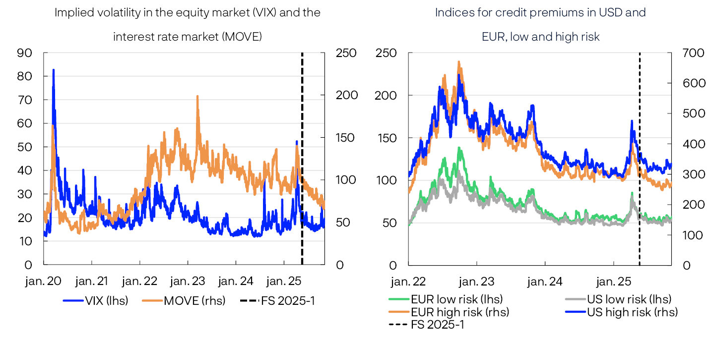
A number of major equity indices have reached new highs, and credit premiums have fallen following the market turbulence this spring (Chart 1.3). The substantial rise in equity prices over the period can partly be explained by slightly higher earnings expectations among firms and higher rate cut expectations in the US.4 However, these factors cannot fully explain the rise in equity prices, indicating that equity risk premiums have fallen. In isolation, this raises the risk of abruptly falling asset prices and rising credit premiums in response to new information.
Global equity indices. January 2024 = 100
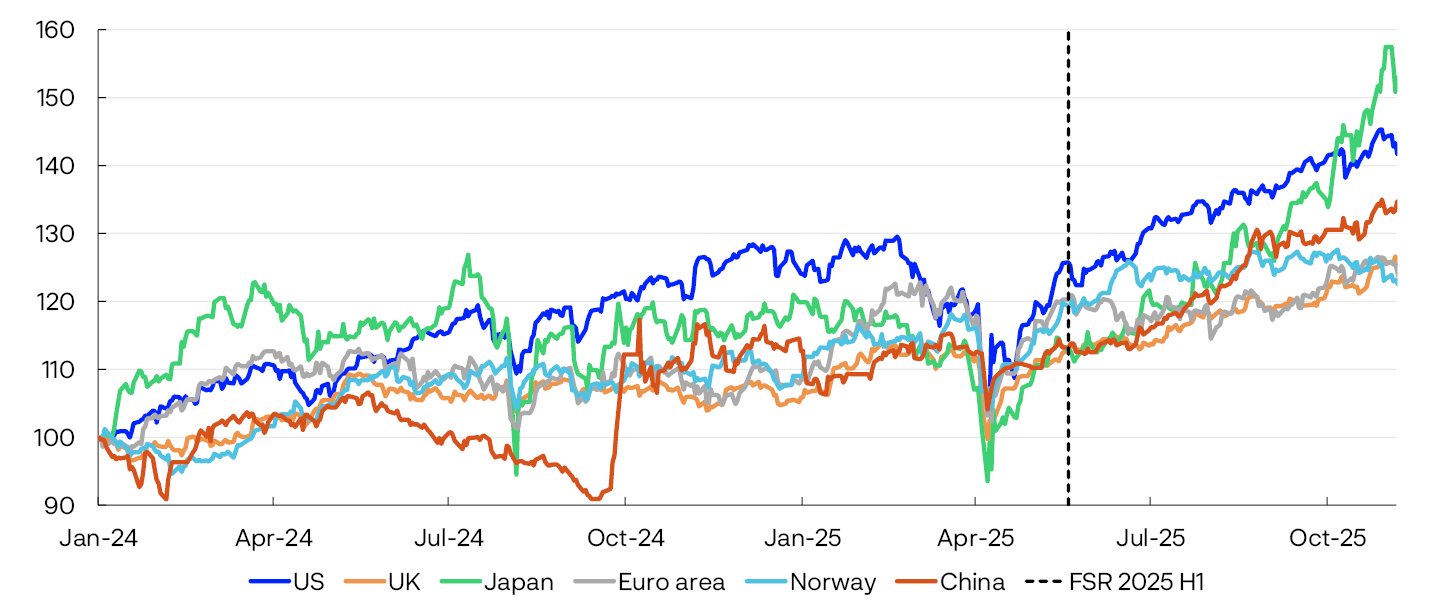
In the US, the rally in equity markets is driven by technology and communication companies, which have announced major investment in, among other things, AI and data centre developments. The seven largest companies in the US S&P500 benchmark index account for a steadily increasing share of market value6, and developments in the index are therefore heavily influenced by a small number of companies in the same sector. Technology shares on Oslo Børs have also surged but make up a relatively small share of the benchmark index. In Norway, energy equities have fallen in pace with lower oil prices, while consumer goods equities have increased.
Turbulence in international financial markets can result in a rise in the risk premiums paid by banks on wholesale funding, both in Norway and in other countries. As Norwegian banks have high credit ratings and are well capitalised, this may better insulate them against international market turbulence. At the same time, much of Norwegian banks’ funding is raised abroad and well-functioning international financial markets are therefore important to them.
The US dollar weakened following market turbulence this spring
The US dollar plays a key role in the global financial system and influences, among other things, conditions for financing and the pricing of risk, also in Norwegian markets. Previously, the US dollar has appreciated during market turbulence and thereby helped dampen the depreciation of US assets owned by US investors. However, in connection with the period of market turbulence this spring, the US dollar depreciated sharply together with an abrupt fall in equity prices. Since then, the decline in asset prices and premiums has been reversed, but the dollar has not appreciated. The IMF highlights several reasons for the dollar depreciation, including concerns over US government finances and political uncertainty.7 Furthermore, the IMF points out that while there has so far been little sign of investors withdrawing from the US, many have strengthened their currency hedging positions to reduce the risk of losses on dollar exposures. The increase in hedging has likely contributed to the dollar depreciation.
Norwegian banks have largely hedged foreign exchange risk. A weakening of the US dollar could nevertheless impact bank liquidity by increasing collateral requirements in currency swaps and requiring them to surrender liquidity to counterparties in these agreements. If the US dollar depreciates sharply and suddenly, collateral requirements are not likely to pose a liquidity challenge to Norwegian banks.
Increased supply and lower demand for long-term government bonds may push up long-term yields
The government bond market is important for financial stability. Government bonds serve, among other things, as a benchmark for other asset prices and as collateral for loans and derivatives transactions. In many countries, banks have large holdings of government bonds. If countries’ credit ratings are downgraded, banks’ credit quality could deteriorate, which may increase banks’ funding costs and result in tighter credit standards for households and firms.
A number of European countries are now increasing defence expenditure sharply. At the same time, expenses related to climate transition and an ageing population are rising, which will likely lead to larger fiscal deficits and an increased supply of government bonds. This may push up the premiums required by investors to hold long-dated rather than short-dated bonds, measured as the term premium. Pressure on government budgets, particularly in highly indebted countries, may erode fiscal space to address future problems and financial downturns.
Other developments may also have contributed to higher term premiums in the government bond market. In recent years, a number of the largest central banks have started to reverse their asset purchase programmes, ie they let their bond portfolios mature and no longer purchase government securities. At the same time, the transition from defined-benefit to defined-contribution occupational pension schemes in a number of European countries has resulted in lower demand from pension funds and insurance companies for long-term government bonds to meet their long-term obligations. Some funds will likely also have to sell significant volumes in a transitional period, which will increase the supply of government bonds.8 The uncertainty related to how lower demand will be balanced against a continued high and increasing supply of government bonds may intensify volatility in fixed income markets ahead and higher long-term yields.
Also in Norway, the transition to defined-contribution pension schemes has reduced the volume of Norwegian pension funds’ holdings of long-term bonds than was previously the case. The shift towards other assets, such as equities and shorter-dated bonds, has been gradual.
Non-bank financial institutions may amplify market turbulence
Important functions in the financial system are performed by non-bank financial institutions (NBFIs)9. They play a key role in channelling capital, sharing risk and contributing to financial stability. These institutions can assume, transform or transfer risk from the banking sector to market participants that are better positioned to manage such risk. Increasing interconnectedness between banks and less regulated NBFIs may, however, be a source of financial system vulnerabilities.
Internationally, NBFIs are playing an increasingly prominent role in the government bond market and in credit intermediation to non-financial corporates. In many countries, including Norway, the total assets held by NBFIs have grown more than the total assets held by banks. So far, direct lending from NBFIs to Norwegian non-financial corporates is limited (see “Who lends to Norwegian non-financial corporates?”).
At the same time, NBFIs have direct connections to banks through ownership of each other’s equity capital and debt instruments or by being counterparties in derivatives transactions (see Section 2.3 in Financial Stability Report 2025 H1. In a crisis, these close connections can amplify market movements and contribute to the transmission of stress to other parts of the financial system. In October, uncertainty about the credit quality and potential losses on securitised US corporate loans, which are held by both banks and NBFIs, led to a fall in global equity markets. This also illustrated the heightened attention in financial markets to connections between banks and NBFIs.
Norwegian banks’ direct exposure to the Norwegian NBFI sector is low compared to banks’ total assets, but the sector is important for banks’ wholesale funding. NBFIs hold, among other things, a substantial share of bonds issued by banks and mortgage companies. Selling pressure may arise if NBFIs, such as hedge funds, need liquidity, for example as a result of substantial collateral requirements in derivatives contracts or large redemptions of fund units. This may lead to a fall in bond prices and amplify market stress, as seen during the pandemic in 2020.
Foreign hedge funds hold an increasing share of covered bonds issued in NOK and use repurchase agreements with Nordic banks to obtain leverage. Leveraging enables the hedge funds to achieve high returns but also makes the funds vulnerable to events that may force them to conduct fire sales of covered bonds. This may lead to stress in the covered bond market, which may spill over to other parts of the credit market (see Financial Stability Report 2025 H1.
Amendments to the regulations for alternative investment funds (AIFs), AIFMD 2.0, allow such funds to engage in lending to consumers and non-financial corporates (see “Regulatory amendments permit alternative investment funds to engage in lending”). A broader range of financing sources can, in principle, strengthen financial stability by spreading credit risk among multiple market participants. On the other hand, lending through AIFs may entail vulnerabilities. Weaker reporting requirements may obscure risk and contribute to reducing transparency in credit markets.
Regulatory amendments permit alternative investment funds to engage in lending
Alternative investment funds (AIFs) are collective investment schemes that are not undertakings for collective investment in transferable securities (UCITS). AIFs pool capital from multiple investors and have a defined investment strategy. AIFs include real estate funds, private equity funds and hedge funds. Most AIFs in Norway are funds that invest capital, but an AIF can also be a private credit fund that provides direct lending. Such funds have grown rapidly in both the US and Europe.1 Private credit has been limited in Norway up to now, partly because funds require a bank or financial institution licence to engage in lending.2
In Norway, AIFs are regulated by the AIF Act, which implements the AIF Directive of 2011. In March 2024, the EU adopted amendments to the AIFM and UCITS directives, and these amendments are often referred to as AIFMD 2.0. The amendments harmonise provisions for lending from AIFs in the European Economic Area and permit lending to both consumers and firms. Member states can prohibit lending from AIFs to consumers. The Ministry of Finance has submitted a consultation proposal prepared by Finanstilsynet on how AIFMD 2.0 should be implemented in Norwegian law.3 Finanstilsynet proposes that Norway should exercise the option to prohibit lending from AIFs to consumers. AIFMD 2.0 will apply in the EU from April 2026 but can only enter into force in Norway upon incorporation into the EEA Agreement. Once the regulations enter into force, the option to provide loans through AIFs will be expanded considerably.
Private credit still accounts for a small share of overall lending globally, and overall risk is therefore considered limited. However, a growing market and forthcoming regulatory changes suggest that future developments should be monitored closely.
1 See eg ECB (2024) Private markets, public risk? Financial stability implications of alternative funding sources and Section 2 in IMF (2024) The Last Mile: Financial Vulnerabilities and Risks.
2 The ELTIF Regulation does, however, permit some forms of long-term loans, and Union Kreditt was first to launch a private credit fund aimed at commercial real estate under this framework in 2024. The European Venture Capital Fund (EuVECA) Regulation and the European Social Entrepreneurship Funds (EuSEF) Regulation also permit lending under certain stipulated terms and conditions.
3 For more information about the consultation process, see news item from the Ministry of Finance dated 8 October 2025 (in Norwegian only).
Stablecoins may give rise to systemic risk further out
Norges Bank is seeing an increasing level of interconnectedness between traditional finance and the cryptoasset market. Stablecoins, which are a part of this market, are growing rapidly and becoming increasingly connected to the traditional financial system. Such developments have contributed to raising awareness of the potential consequences for financial stability.
Most stablecoins are pegged to the US dollar and are used, among other things, as a store of value and for money transfers in countries with less well-functioning money and payment systems. This has led to concerns over currency substitution in favour of the US dollar in such countries and may weaken the effect of national policy instruments in foreign exchange, money and capital markets.10
Stablecoins are backed by bank deposits and government securities to maintain a stable value relative to the reference asset. However, if confidence is lost, stablecoins may face a redemption run. A right to redeem the stablecoin for the nominal value of the reference currency may amplify vulnerabilities as users will require early redemption while the collateral is still sufficient. Fire sales of underlying assets may lead to a fall in prices and liquidity stress that could spill over to other markets. Wider adoption may also change banks’ funding structure if retail bank deposits are replaced to a greater extent by few and larger deposits from stablecoin issuers. Few deposits from some professional market participants may lead to more volatile financing and potentially reduce banks’ capacity to provide lending to households and firms.
To date, the exposure to cryptoassets in banks and other financial institutions appears limited. The IMF emphasises that the potential systemic effects depend on whether stablecoins continue to grow.11 Stablecoins in NOK have not yet been issued, but banks in the US and Europe have shown an interest in issuing stablecoins in EUR and USD, both individually and in collaboration, see “Increased interest in stablecoins triggers need for regulation”.
1 See press release from the ESRB’s General Board meeting on 25 September 2025: Outcomes of the 59th General Board meeting of the European Systemic Risk Board – 25 September 2025
2 Based on Norges Bank’s Systemic Risk Survey from October 2025. A selection of participants in the Norwegian financial system take part, and the responses reflect the risk assessments at the time the survey was conducted.
The chart shows the source of risk considered most likely in the Norwegian financial system according to the respondents.
3 Left panel:
Period: 1 January 2020 – 5 November 2025.
Right panel:
Period: 1 January 2022 – 5 November 2025.
4 Market participants’ earnings expectations are consensus estimates for annual earnings from Bloomberg.
5 Period: 1 January 2024 – 5 November 2025.
6 The seven largest technology companies are often called “the Magnificent 7” and now account for around 35% of the market value of the S&P 500 index. They are currently Nvidia, Microsoft, Apple, Alphabet/Google, Amazon, Meta and Broadcom.
8 For example, all pension schemes in the Netherlands will be converted to defined-contribution models over the next two years. This may trigger a need for Dutch pension funds to sell a substantial volume of long-term European government bonds.
9 NBFI is an abbreviation for “non-bank financial Institutions” or “non-bank financial intermediation” and includes insurance companies, investment funds and assets managers, such as hedge funds.
1.2 Norwegian banks are resilient
Banks are profitable and credit losses are low
International shocks and market stress may have consequences for the funding conditions of Norwegian banks. Banks’ funding markets have functioned well since the May Report. Risk premiums on banks’ wholesale funding have fallen somewhat, and deposit-to-loan ratios are stable. Norwegian banks satisfy capital and liquidity requirements by a solid margin.
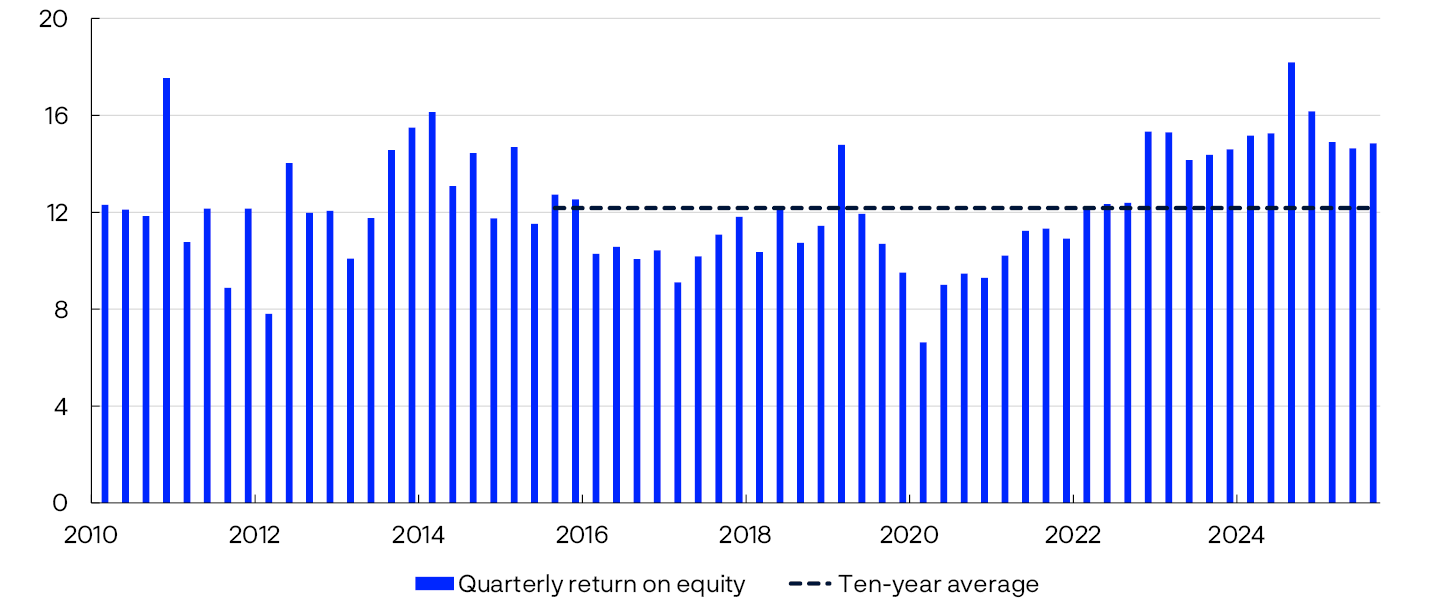
Current earnings are banks’ first line of defence against losses. Return on equity for the large Norwegian banks has been high over the past three years (Chart 1.4). This increase in profitability has been mainly driven by increased net interest income and low losses. Higher net interest income reflects higher interest rate levels in recent years.12 The policy rate forecast from Monetary Policy Report 3/2025 indicates a lower interest rate level in the coming years. Combined with a decline in banks’ interest margins, this will pull down net interest income and thus banks’ profitability.
Return on equity after tax for large banks. Percent
Banks’ total credit losses have remained low and in line with 2024 levels (Chart 1.5).
Loan losses as a percentage of gross loans to customers
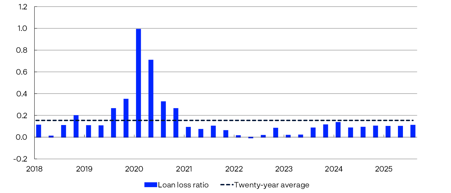
Banks’ corporate credit losses have also remained low. Norges Bank expects continued low construction activity to contribute to somewhat higher corporate default rates and credit losses in real estate development over the coming year (for more details, see Section 3). CRE prospects are stable. If employment were to fall markedly and rental income developments in the CRE sector prove markedly weaker than expected, banks could face substantial losses.
As a whole, Norwegian banks have moderate direct exposure to export-oriented industries, ie those directly impacted by trade restrictions. However, there are regional variations in industry structure, and the exposures of banks with different regional affiliations can vary. Lending to the fisheries and aquaculture sector, which can be affected both directly and indirectly by higher tariffs, accounts for around 6% of total bank corporate lending. See Section 3.2 for a detailed discussion of the impact on the fisheries and aquaculture sector.
Losses on loans to households are low. Looking ahead, higher real household income and lower interest rates are expected to strengthen debt-servicing capacity, and the loss rate on household exposures is expected to remain at a low level.
Banks are solid
Common Equity Tier 1 (CET1) ratios are well above total capital requirements and above banks’ own target ratios. Looking ahead, continued high profitability and low losses are expected to keep banks’ capital adequacy ratios at a high level. The amendments to the Capital Requirements Regulation (CRR III), which entered into force on 1 April 2025, mean that banks using the standardised approach (SA) will have lower capital requirements for low-risk exposures. This has increased SA banks’ capital adequacy ratios. So far, IRB banks are less affected by CRR III. The increase of the risk weight floors for IRB banks from 20% to 25% for residential mortgages has, in isolation, somewhat reduced IRB banks’ capital requirements.
The stress test in Financial Stability Report 2025 H1 shows that, on the whole, the largest Norwegian Banks are capable of absorbing large losses while maintaining lending to households and firms, and thereby will not contribute to amplifying an economic downturn.
Households and firms have ample access to credit
Norwegian banks’ financial strength gives them the flexibility to extend loans to creditworthy firms and households, even in the event of market stress and higher losses. In Norges Bank’s lending survey for 2025 Q3, banks reported unchanged credit standards, somewhat stronger household credit demand and slightly weaker corporate credit demand. Banks expect unchanged credit standards and credit demand in Q4. This autumn, bond market activity has been high, and credit premiums for investment-grade firms are close to the average for the past decade. In Norges Bank’s overall assessment, households and firms have ample access to credit.
12 Policy rate hikes increase banks’ interest income more than interest expenses because banks have more interest-bearing assets than interest-bearing liabilities (equity effect). In addition, banks often raise average lending rates more than average deposit rates (interest margin increase).
13 Period: 2010 Q1 – 2025 Q3.
Figures for the six largest Norwegian-owned banking groups. Annualised.
For comparability, the sample has been adjusted retrospectively for major mergers/acquisitions; ie for periods prior to a merger/acquisition, figures for the merged banks have been included.
14 Period: 2018 Q1 – 2025 Q3.
All banks and mortgage companies in Norway. Annualised. Branches and subsidiaries abroad are not included.
Who lends to Norwegian non-financial corporates?
Firms have two main sources of debt financing. They can borrow directly from a financial institution, or they can issue wholesale funding in the form of bonds and short-term papers. Historically, banks have been the most important source of direct lending to firms.
After the 2008–2009 financial crisis, banking regulations were tightened in many countries, leading to a marked rise in direct lending from non-bank financial institutions (NBFIs), particularly in the US. In Europe, growth has been more moderate and most extensive in the UK.
Norwegian non-financial corporates borrow little from Norwegian NBFIs
Domestic credit (C2) and total credit (C3) indicators published by Statistics Norway provide the basis for the mapping of credit to Norwegian non-financial corporates.1 The indicators show firms’ stock of credit from different sources in Norway and abroad.
At the end of 2025 Q2, Norwegian firms’ total debt amounted to NOK 3 155bn (Chart 1.A), 59% of which was borrowed from Norwegian banks. Firms also borrow from other Norwegian lenders, such as pension companies and insurance firms, finance companies and public institutions.2 At the end of 2025 Q2, these loans accounted for approximately 5% of total corporate debt. In addition, firms hold some foreign debt, primarily from credit institutions and market-based bond financing.
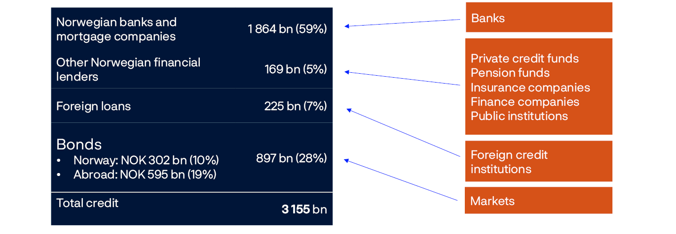
At the end of 2025 Q2, bonds accounted for approximately 28% of total corporate debt. Around two-thirds of this debt is issued abroad, often in another currency than NOK. Large firms in particular participate in foreign bond markets. Around one-third of bond debt abroad is issued by firms in the petroleum and international shipping sectors.
The distribution of corporate debt has remained relatively stable over time (Chart 1.B, left panel). The share of debt issued by banks has increased somewhat over the past decade. Growth in bond debt issued in Norway was rapid during the pandemic but has slowed in recent years (right panel), largely reflecting lower issuance volumes and a considerable wave of CRE debt maturities. Growth in the issuance of foreign loans and bonds has varied, but increased in total as much as lending by Norwegian banks since 2015 (right panel).
Total credit to non-financial corporates

In contrast to global developments, direct lending from other Norwegian lenders, including NBFIs, has declined somewhat since the peak in 2020 (Chart 1.C). Most of these loans are issued by finance companies that typically provide leasing, factoring and the like. Many of these financial institutions are owned by banks. State lending institutions such as Innovation Norway and Eksportfinans are also important sources of such loans (Chart 1.C).
In billions of NOK

Approximately 1% of corporate credit comes from market participants that are considered NBFIs, ie life and non-life insurance companies and pension funds. Life insurers account for most of the lending.6 Microdata from the Norwegian Tax Administration show that direct lending from NBFIs is largely from a small number of large lenders and to a few borrowers, particularly CRE firms.
In Norway, direct lending from private NBFIs still only accounts for a small share of corporate financing. Amendments to the Alternative Investment Fund Managers Directive (AIFMD II) may facilitate higher lending activity among private Norwegian NBFIs in the years ahead (see discussion in “Regulatory amendments permit alternative investment funds to engage in lending”).
1 Norges Bank has retrieved data from Statistics Norway for firms’ foreign debt by credit source. Total foreign debt is somewhat lower in these data than total foreign debt in official statistics. Nevertheless, developments are roughly the same.
2 C2 does not include loans from investment funds other than bonds and short-term paper. According to Statistics Norway’s financial accounts, loans from investment funds to non-financial corporates amounted to NOK 54bn in 2025 Q2. However, these financial accounts have limited data for these funds and loans from investment funds to non-financial corporates are used as a balancing item to achieve a better alignment between financial assets and liabilities. This leads to considerable uncertainty regarding actual amounts.
3 Figures as at 30 June 2025.
4 Left panel:
Period: 2015 Q2 – 2025 Q2.
Credit to non-financial corporates from banks and mortgage companies, other Norwegian financial lenders, foreign loans, and bonds issued abroad.
Right panel:
Period: 2015 Q1 – 2025 Q2.
Relative developments in credit to non-financial corporates from banks and mortgage companies, other Norwegian financial lenders, foreign loans, and bonds issued abroad.
5 Period: 2015 Q2 - 2025 Q2
Lending to non-financial corporates that is not from Norwegian banks and mortgage companies, abroad or from bond debt according to Statistics Norway’s data for household and non-financial corporate lending (C2).
6 See footnote 2 on loans from investment funds other than bonds and short-term paper.
Key vulnerabilities in the Norwegian financial system
The economy is regularly exposed to shocks that affect both the real economy and the financial system. Promoting financial stability means ensuring sufficient financial system resilience to absorb such shocks. The financial system should contribute to stable economic developments by channelling funds and offering savings products, executing payments and distributing risk efficiently. Systemic risk is the risk of disruption to the financial system’s ability to perform these functions.
The level of systemic risk depends on a number of factors. The risk of economic shocks, such as geopolitical tensions, pushes up systemic risk. Financial system vulnerabilities further increase systemic risk. Chart 1.D summarises Norges Bank’s key assessments of Norwegian financial system vulnerabilities.

The high indebtedness of many households is a key vulnerability.
Debt-to-income (DTI) ratios are high compared with other countries. This vulnerability has built up over time as debt levels rose more than household income over an extended period. In the years preceding the pandemic, debt growth slowed and kept more closely in pace with income growth. In recent years, debt growth has been slower than income growth. Debt-to-income ratios have declined broadly across households and most of all for those with the highest DTI ratios. In Norges Bank’s overall assessment, Norwegian household vulnerabilities related to high debt have been somewhat reduced. Vulnerabilities may increase again if looser financial conditions result in rapidly rising house prices and debt. For a more detailed discussion of households’ vulnerabilities, see Section 2.
Another key vulnerability is banks’ high CRE exposure. Higher financing costs have reduced CRE profitability, and lower property values have weakened solvency. However, high employment and growth in rental income enable most CRE firms to cover high interest expenses with current earnings. Nevertheless, developments ahead remain uncertain. If interest rates and risk premiums rise markedly or rental income developments prove markedly weaker than envisaged, profitability and property values will weaken. See Section 3 for a more detailed discussion of the CRE sector.
Furthermore, banks in Norway are interconnected through interbank exposures and have common or similar securities in their liquidity reserves (see Financial Stability Report 2025 H1). Covered bonds account for a large part of banks’ liquidity reserves. If a number of banks need liquidity and have to sell such a large quantity of covered bonds that their value falls, the value of covered bond holdings in the liquidity reserves of all other banks will also fall. Cross-holdings of bonds mean that banks fund other banks. If banks are no longer buyers of covered bonds during market stress, this could weaken the possibility of other banks issuing new covered bond funding and could more easily lead to liquidity problems spreading and becoming self-reinforcing.
Digitalisation makes the financial system more efficient but also gives rise to vulnerabilities. Concentration, complexity and interconnectedness may amplify the consequences of a cyberattack that then spreads rapidly and widely across the financial system. If the overall consequences become sufficiently extensive, financial stability could be threatened. With the increased severity of the current threat landscape, consideration must be given to the fact that even well-protected systems can become unavailable. Adequate contingency arrangements are important for managing such serious situations (see Financial Infrastructure Report 2025).
Moreover, banks’ substantial exposures to sectors that are particularly vulnerable to climate transition are a financial system vulnerability. The Norwegian business sector must adapt to climate change and the use of new forms of energy. There is considerable uncertainty about the cost of such a transition, and some firms may see their earnings weaken. If many firms are adversely affected, this may result in higher bank losses. In addition, more extreme weather events can also increase housing-related costs and thereby impact household resilience (see box in Section 2).
However, the financial system can be designed to be more resilient to shocks. In response to financial system vulnerabilities, a number of measures have been introduced to strengthen resilience, including requirements for banks’ solvency, liquidity and credit standards.
Increased interest in stablecoins triggers need for regulation
Stablecoins are cryptoassets that aim to maintain a stable value against a reference asset, most often the US dollar. Issuers maintain the value against the reference asset by securing the coin on traditional financial assets such as securities and bank deposits. Even though stablecoins are currently used as a store of value and for payments within the crypto ecosystem, the range of applications are under development.1
Attributes such as immediate settlement and low transaction costs, particularly for cross-border payments, have boosted global interest in stablecoins. The market value of stablecoins remains low compared with traditional finance and the wider crypto market, but their value has grown rapidly. Their value has increased from USD 3bn in 2019 to over USD 300bn so far in 2025.
A number of major jurisdictions have established special regulatory frameworks for stablecoins. The European Markets in Crypto-Assets (MiCA) Regulation entered into force in Norway under the new Cryptoassets Act on 1 June 2025.2 The legislation applies to cryptoasset issuers and service providers and requires information and documentation for issuances and sales. The MiCA Regulation delegates certain licensing, supervisory and monitoring tasks to the European Central Bank (ECB) and national central banks. On 18 July 2025, the US GENIUS Act was the first federal stablecoin legislation to be adopted.3 GENIUS is similar to MiCA, and a key objective is strengthening the global prominence of the US dollar through the increased use of stablecoins and demand for US government securities. In the UK, stablecoin regulation, with many similarities to MiCA, is also in the pipeline, and the Bank of England has endorsed the possibility of a role for stablecoins in the monetary system.4
Stablecoins are used globally, with many issuers operating in a number of jurisdictions. Stablecoins are designed to be fungible, regardless of where they are issued. Stablecoins issued in multiple jurisdictions (multi-issuer stablecoins) may lead to holders seeking redemption in jurisdictions offering more favourable terms, thereby concentrating vulnerabilities in well-regulated markets if there is a loss of confidence. The ESRB has recommended implementing measures to limit risk related to stablecoins issued in multiple jurisdictions. 5
Stablecoin regulation is still not sufficiently developed to prevent regulatory arbitrage. According to a report from the Financial stability Board (FSB) in October 2025, even though many jurisdictions have established regulatory frameworks for stablecoins, a fair amount of work remains to meet the FSB’s recommendations for regulating global stablecoin arrangements. This highlights the need for further international cooperation to secure financial stability
1 For more details on stablecoins, see: “Stronger interconnections between cryptoassets and traditional finance” in Financial Infrastructure 2025.
2 For more details on Norwegian cryptoasset regulation, see Kryptoeiendelsloven (MiCAR). (Norwegian only).
3 See Fact Sheet: President Donald J. Trump Signs GENIUS Act into Law – The White House.
4 See speech by Sarah Breeden Not just token gestures.
5 See Recommendation of the European Systemic Risk Board of 25 September 2025 on third-country multi-issuer stablecoin schemes (ESRB/2025/9).
2.1 Debt-to-income ratios decline further
Many Norwegian households have high debt-to-income (DTI) ratios, and Norges Bank has long considered this high debt to be a key vulnerability in the Norwegian financial system. Historically, household default rates have been low, even in downturns. At the same time, high debt levels, especially when combined with low liquidity, can increase the risk of sharp consumption cutbacks if interest rates rise, household income is reduced or house prices fall markedly. Such cutbacks can affect firms’ earnings and in turn lead to higher corporate credit losses among banks.
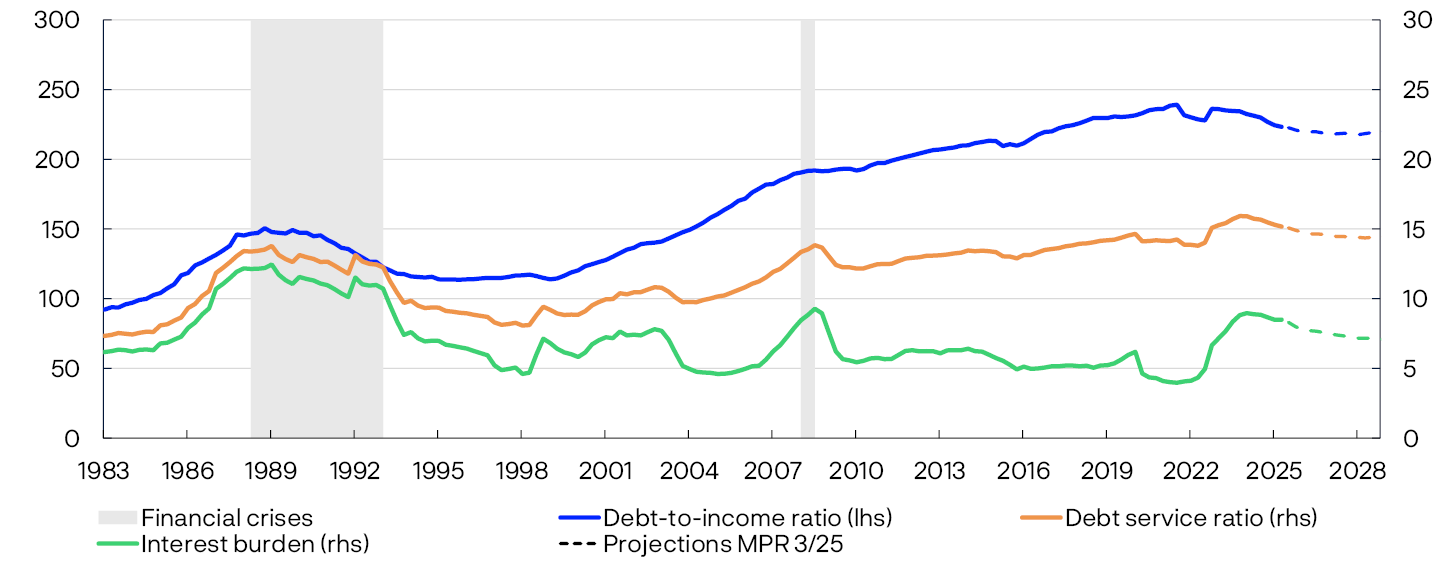
Norwegian household DTI1 ratios rose over many years and are high both historically and compared with other countries (Chart 2.1). Over the past four years, the overall household DTI ratio has levelled off and declined somewhat. Household debt service ratios and the interest burden have declined over the past year, following considerable increases in pace with the rise in interest rates.
According to Finanstilsynet’s (Financial Supervisory Authority of Norway) residential mortgage lending survey for 2025, DTI ratios increased somewhat with new mortgages, and a higher share of new mortgages are issued with loan-to-value (LTV) ratios close to 90%. Developments must be viewed in the light of the increase in the Lending Regulations’ maximum LTV ratio requirement at the turn of the year from 85% to 90%. The survey also shows that the share of loans granted to borrowers with low liquidity when interest rate stress tests are considered has declined after increasing for a number of years.2
Looking ahead, DTI ratios are expected to decline slightly further (see Chart 2.1 and Monetary Policy Report 3/2025). A falling DTI ratio means that income rises faster than debt.
Percent
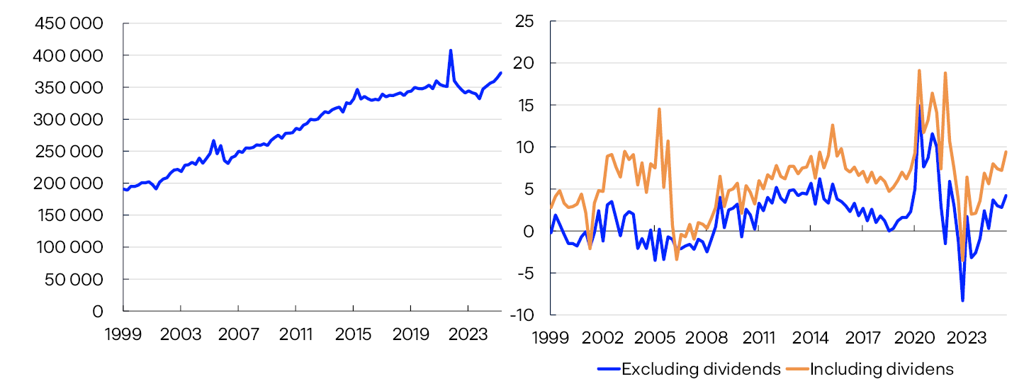
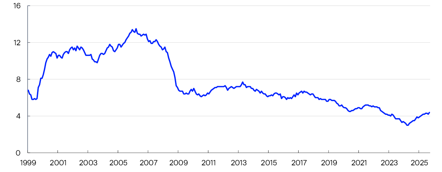
Following a decline in 2022 and 2023, real household disposable income rose rapidly from the start of 2024 (Chart 2.2, left panel). In 2024, the rise in household real disposable income was the sharpest in over a decade. The saving ratio has also moved up again after declining in 2022 (Chart 2.2, right panel). At the same time, household credit growth has picked up somewhat over the past year, with a twelve-month rise of 4.4% in September. This acceleration followed a period of moderating growth, and credit growth remains lower than in the pre-pandemic years (Chart 2.3). According to the banks in Norges Bank’s Survey of Bank Lending, residential mortgage demand increased somewhat in 2025 Q3, while unchanged demand is expected in Q4.
Real disposable income. In millions of 2015 NOK/ Saving ratio. Percent
5Domestic loan debt. Transactions. Twelve-month change. Percent
Household consumer debt increased somewhat in 2022 and 2023, but credit growth has declined over the past two years. At the same time, it has been observed that while credit card usage has increased, interest-bearing credit card debt – ie unsettled credit card debt that accrues interest – has declined since 2022.
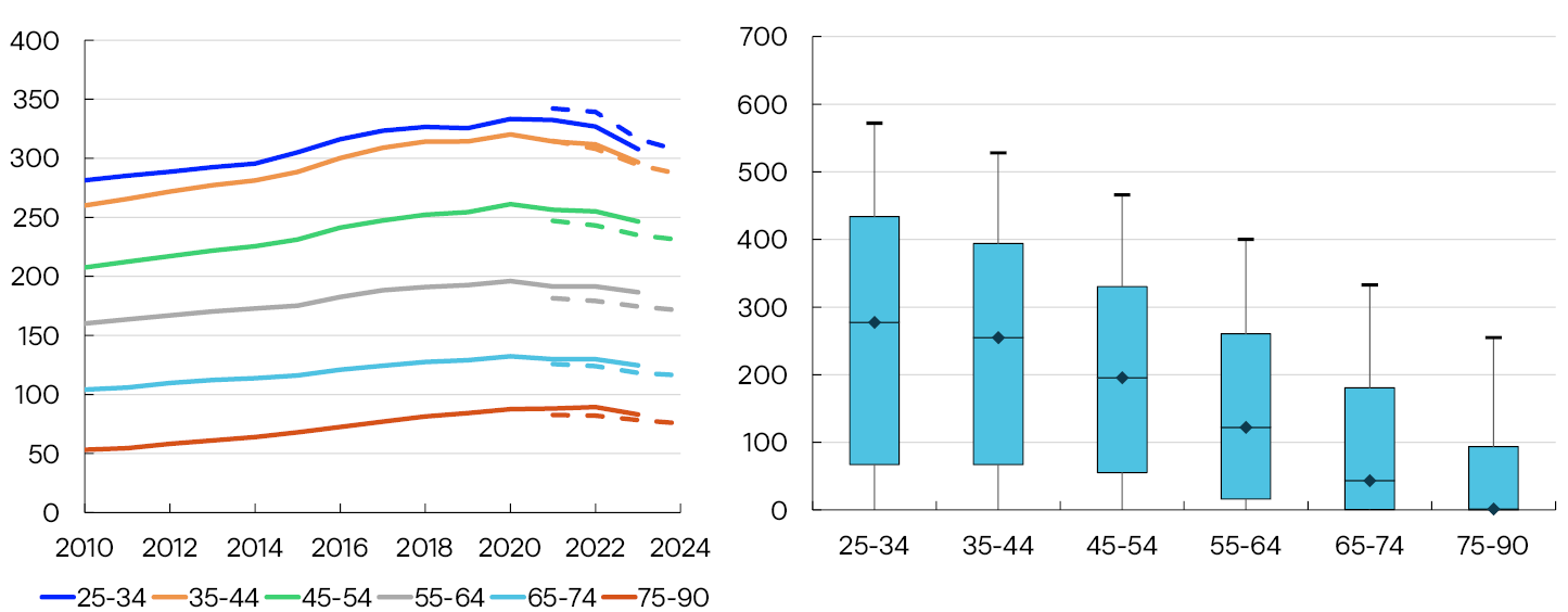
The decline in household DTI ratios is broadly based
Norwegian households have historically accumulated substantial debt, owing primarily to home purchases early in life. DTI ratios therefore vary considerably between households in different age groups (Chart 2.4, left panel). In recent years, DTI ratios have levelled off and declined in all age groups. Since 2021, the decline has been most pronounced among households under the age of 35, which also have relatively high DTI ratios. At the same time, there are wide differences in DTI ratios within each age group (Chart 2.4, right panel). In the 25–34 age group, 10% of households had DTI ratios higher than close to six times after-tax income in 2024. The median ratio in this age group was approximately three times after-tax income. There is also a large portion of the 35–44 age group with relatively high debt levels. Both the differences within these age groups and the percentage with high debt levels decline markedly with age.
Debt as a share of after-tax income by age group. Percent
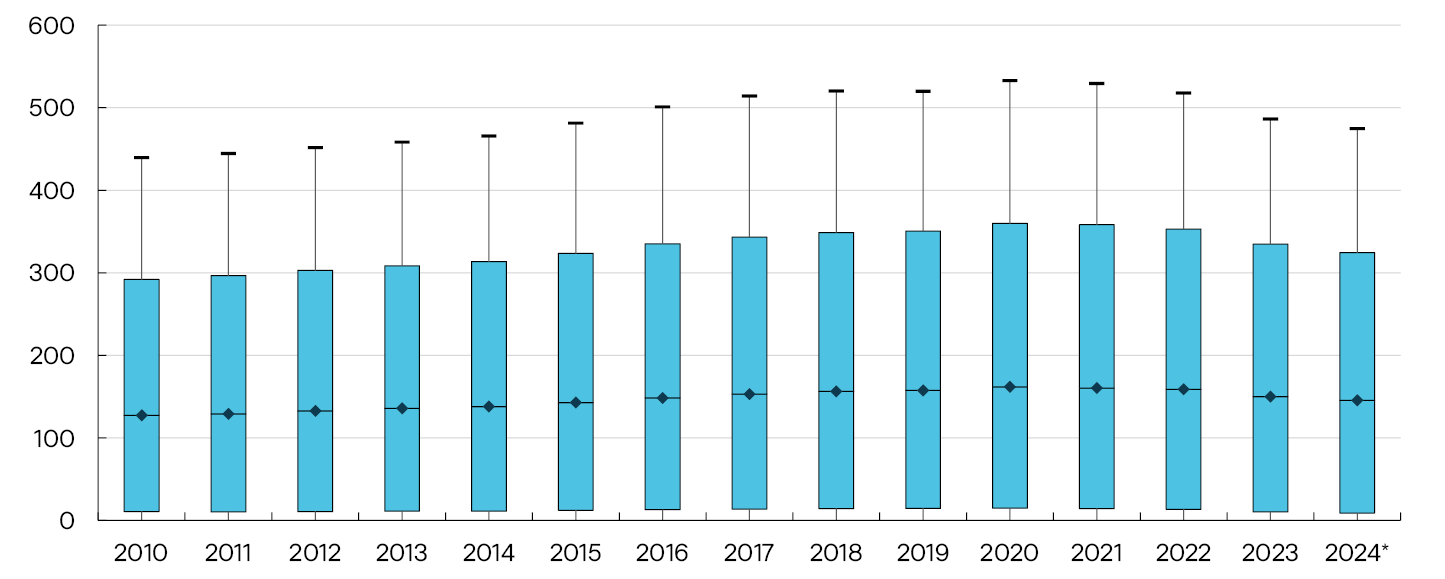
The overall DTI ratio started to decline in 2022, and in 2024, the median DTI ratio was approximately 150% (Chart 2.5). The decline has been most pronounced among households with the highest DTI ratios. This is evident in the chart, which shows that the top of the distribution (90th percentile) has fallen more than the median.
Debt as a share of after-tax income. Percent
Lower household DTI ratios lead to somewhat lower household vulnerability
The high level of household debt is a key financial system vulnerability, particularly as it increases the risk of sharp consumption cutbacks if interest rates rise, household income is reduced or house prices fall markedly. Norges Bank’s assessment is that the broad-based decline in household DTI ratios has reduced this vulnerability somewhat.
In connection with this Report two analyses have been conducted to shed light on the consumption channel described above (see “Housing-related costs may increase due to more frequent extreme weather events” and “Households with high debt-to-income ratios have reduced consumption the most in response to higher interest rates”).8 The first analysis focuses on how households have adjusted their consumption in the period of higher interest rates and rapid inflation. The analysis shows that highly indebted households have reduced consumption more than those with low DTI ratios. The second analysis focuses on how households adjust consumption in response to a sharp fall in house prices. Again, the analysis shows that households with high DTI ratios reduce their consumption more than those with low ratios.
These findings are in line with existing research.9 The fact that household DTI ratios have now declined, and that the decline has been most pronounced among the households with the highest debt, may therefore dampen consumption cutbacks in response to future interest rate hikes or marked falls in home prices.
1 Debt as a share of disposable income.
2 Finanstilsynet’s definition of low liquidity is that the borrower has a monthly buffer of between NOK 0 and NOK 4000 in accordance with the interest rate stress test.
3 Period: 1983 Q1 – 2028 Q4. Projections from 2025 Q3 for MPR 3/25.
The debt-to-income ratio is debt as a share of disposable income. Disposable income is income after tax and interest expenses.
The debt service ratio is interest expenses and estimated principal payments as a share of after-tax income.
The interest burden is interest expenses as a share of after-tax income.
4 Period: 1999 Q1 – 2025 Q2.
Real disposable income is a measure of households’ purchasing power, adjusted for inflation. It shows the income households are left with after paying interest, taxes, pension contributions, remittances and transfers to non-profit organisations.
The saving ratio is savings as a share of disposable income and is shown here both including and excluding dividends.
5 Period: January 1999 – September 2025.
6 Left panel:
Period: 2010–2024.
Debt-to-income ratio is debt as a share of after-tax income. The chart shows total debt divided by total income. The grouping into age groups is based on the age of the main income earner. Households where the main income earner is self-employed are excluded. Households in the top percentile of net wealth are also excluded. Data from the tax assessment are shown by the dotted lines and are estimates based on household composition from the previous year.
Right panel:
Period: 2024.
The debt-to-income ratio is debt as a share of after-tax income. The grouping into age groups is based on the age of the main income earner. Households where the main income earner is under 25 years, over 90 years, or self-employed are excluded. Households in the top percentile of net wealth are also excluded. The boxplots show the 10th, 25th, 50th, 75th, and 90th percentiles (marked, respectively, by the lowest horizontal line along the black vertical line, the bottom of the blue box, the diamond, the top of the blue box, and the top vertical line along the black line). The figures are estimates generated from the tax assessment based on household composition from 2023.
7 Period: 2010–2024.
Debt-to-income ratio is debt as a share of after-tax income. Households where the main income earner is under 25 years old, over 90 years old, or self-employed are excluded. Households in the top percentile of net wealth are also excluded. The boxplots show the 10th, 25th, 50th, 75th, and 90th percentiles (marked, respectively, by the lowest horizontal line along the black vertical line, the bottom of the blue box, the diamond, the top of the blue box, and the top vertical line along the black line).
The figures for 2024 are estimates generated from the tax assessment based on household composition from 2023.
8 See Guldbrandsen, M. A. H., S. L. Nilsen and E. S. Njølstad (2025) “Revisiting imputed consumption expenditure during the recent tightening cycle in Norway”, Staff Memo 13/2025. ; Aastveit, K. A., Böjeryd, J., Gulbrandsen M. A. H., Juelsrud, R. E., and Roszbach, K. (2025): “What Do 12 Billion Card Transactions Say About House Prices and Consumption?” Working Paper 15/2025. Norges Bank.
9 See eg Ahn, Galaasen and Mæhlum (2024) “The Cash-Flow Channel of Monetary Policy – Evidence from Billions of Transactions” Working paper 20/2024, Norges Bank, Holm, Paul and Tischbirek (2021) “The Transmission of Monetary Policy under the Microscope”, Journal of Political Economy, 129(10), pp 2861–2904 and Fagereng, Onshuus and Torstensen (2024) “The consumption expenditure response to unemployment: Evidence from Norwegian households”, Journal of Monetary Economics.
2.2 Most households have adequate
debt-servicing capacity
Households’ discretionary income fell further in 2024
The combination of higher interest rates and high inflation in the years after the pandemic has left households with a smaller share of their income after taxes, normal living expenses and interest and principal payments have been paid (Chart 2.6).10 This buffer is referred to as discretionary income. Calculations show that the average discretionary income of Norwegian households amounted to approximately 40% in 2024, down from about 45% in 2021. This decline has mainly been driven by higher interest expenses and food prices. On the other hand, strong nominal wage growth and lower principal payments owing to the repayment of self-amortising mortgages have cushioned the decline in discretionary income. Despite higher expenses, most households are able, by an ample margin, to service debt and cover ordinary living expenses out of current income.11
Expenses as a share of after-tax income. Average. Percent

However, an increasing number of households have relatively low levels of discretionary income. The share of households with discretionary income below 40% of their after-tax income has risen steadily since 2021 (Chart 2.7). The share of households with discretionary income of at least 50% of their after-tax income was close to 30% in 2024, broadly the same as in 2023.13
Share of households within different intervals of discretionary income as a share of after-tax income. Percent

Very few households are at risk of defaulting on debt
Approximately 5% of households had negative estimated discretionary income in 2024, slightly lower than in 2023 (Chart 2.7). In order to meet their obligations, these households must either maintain a lower consumption level than assumed in this analysis,15 have unregistered income, draw on accumulated savings or receive transfers from others. In the event of payment problems, they can ask their bank for interest-only periods. Having negative discretionary income does not necessarily mean that a household will default on its debt.
To determine which households are at real risk of debt default, a margin factoring in these possible adjustments is calculated. A negative margin means that a household is not in a position to pay interest unless it reduces consumption to below a normal level.16 Approximately 1.2% of households had negative margins in 2024 (Chart 2.8),17 accounting for approximately 2.2% of overall household debt. The share of households with negative margins is higher than in 2022, but lower than in 2023. Looking at the share of debt held by these households, the same pattern emerges. These calculations are in line with the low residential mortgage default figures.
Share with a negative margin. Percent
Housing-related costs may increase ahead and reduce discretionary income
Households’ debt-servicing capacity depends to a large extent on the size of their discretionary income, and Norges Bank therefore closely monitors factors that can impact this income. Since the pandemic, higher interest and food expenses in particular have reduced discretionary income. One factor that could potentially reduce discretionary income ahead is higher housing-related costs given higher physical climate risk. The rise in home insurance premiums has outpaced consumer price inflation in recent years and was particularly sharp between 2023 and 2024 following the extreme weather event “Hans”. Municipal fees have also increased, partly due to changes in weather conditions resulting in wear and tear on public infrastructure. If changes in weather conditions continue to lead to higher public fees and insurance premiums, a rise in housing-related costs can be expected (see “Lower housing affordability in urban areas: how do first-time buyers respond?”). When calculating discretionary income, housing-related costs are found to amount to a relatively modest share of household after-tax income. At the same time, such costs have increased substantially in other countries. Natural disaster insurance and preventive measures may help dampen the risk of similar developments in Norway and thereby limit the reduction in household discretionary income.
10 Note that households are limited to owner-occupiers, which means that some of the households with the smallest margins are excluded.
11 Finanstilsynet’s residential mortgage lending survey for 2025 shows that the share of loans granted to borrowers with low liquidity when interest rate stress tests are considered has declined after increasing for a number of years.
12 Period: 2020–2024.
The sample only includes households that own their own home.
Self-employed persons and homeowners where the main income earner is under 20 or over 90 years old are excluded. Those with the top 1% highest and lowest incomes, and those with the top 1% highest financial assets, are also excluded.
Discretionary income is the money remaining after households pay taxes, cover debt expenses and normal living expenses. Debt expenses include interest payments and also, if the LTV ratio is over 60%, principal payments.
Normal living expenses cover food, other essential consumption and housing expenses. Food and other essential consumption are based on household size and SIFO’s reference budget. Housing expenses include municipal fees, property tax and insurance. In addition, electricity expenses are estimated based on the home’s size, type, and electricity zone.
13 Owing to an error in underlying data used in Financial Stability Report 2024 H2, Chart 2.5 was misleading. For example, the share of households with discretionary income below 30% of after-tax income should have been around 40% rather than 7%, and the share with more than 50% of their income as discretionary income should have been around 25% instead of 60%.
14 Period: 2020–2024.
The sample only includes households that own their own home.
Self-employed persons and homeowners where the main income earner is under 20 or over 90 years old are excluded. Those with the top 1% highest and lowest incomes, and those with the 1% highest financial wealth, are also excluded.
Discretionary income is the money remaining after households pay taxes, cover debt expenses and normal living expenses. Debt expenses include interest payments and, if the loan-to-value ratio is over 60%, also principal payments.
Normal living expenses cover food, other essential consumption and housing cushioned. Food and other essential consumption are based on household size and SIFO’s reference budget. Housing cushioned include municipal fees, property tax, and insurance. In addition, electricity expenses are estimated based on the home’s size, type and electricity zone.
15 The Consumption Research Norway (SIFO) reference budget is included as a basis. The budget shows the cost of maintaining an acceptable level of consumption – a level that is generally considered reasonable – for the household in question. Nevertheless, this is not a minimum budget, and certain households may therefore consume less when finances are tight.
16 When calculating the margin, it is assumed that banks will grant interest-only periods to households facing payment difficulties if the LTV ratio is below 60%. Borrowers can also draw on some of their accumulated savings to cover ordinary living expenses and interest payments. This means drawing on deposits and funds, as well as the possibility of increasing the LTV ratio if it is below 60% (see Lindquist, Solheim og Vatne (2022): “Norwegian homeowners’ debt-servicing capacity is adequate”, Staff Memo 8/2022, Norges Bank.
17 This corresponds to approximately 20 000 households.
18 Period: 2020–2024.
The sample only includes households that own their own home.
Self-employed persons and homeowners where the main income earner is under 20 or over 90 years old are excluded. Those with the top 1% highest and lowest incomes and those with the top 1% highest financial wealth, are also excluded.
A negative margin indicates when the household is no longer able to service its debt without having to reduce consumption below a normal level.
When calculating the margin, households with payment difficulties are assumed to be granted an interest-only period by the bank if the loan-to-value ratio is below 60%. The borrower may also use some of their savings to cover normal expenses and interest payments. This includes drawing on deposits and funds, as well as the possibility to increase the loan-to-value ratio if the loan is less than 60% of the value of the home.
2.3 Households’ liquid buffers have increased over a long period, but have been reduced somewhat in recent years
Bank deposits are the most common form of savings for households
Bank deposits are the most liquid of households’ accumulated savings and the dominant form of financial wealth for most households (Chart 2.9).19 Bank deposits account for more than 90% of the financial wealth of half of Norwegian households, while just over a third of households only have bank deposits. At the same time, financial wealth has become slightly more diversified in recent years as a result of more households saving in funds and other financial assets. Some of these investments, such as broad-based index funds, are liquid and relatively simple to sell to improve household liquidity.
Bank deposits’ share of financial wealth. Percent

Households’ liquid buffers have been somewhat reduced as a share of income in recent years
Liquid buffers improve households’ ability to handle unforeseen expenses or a loss of income. After having risen for several years and surged during the pandemic, bank deposits as a share of after-tax income declined in pace with higher interest rates and high inflation (Chart 2.10, left panel). In 2023, the share returned to around pre-pandemic levels. For the median household in 2023, deposits amounted to slightly more than 30% of annual after-tax income. Preliminary data from the Norwegian Tax Administration and aggregated figures from Statistics Norway’s financial sector accounts indicate that the share has fallen slightly further in 2024 and 2025.
Bank deposits’ share of after-tax income. Percent / Liquid assets’ share of after-tax income. Percent
If fund units and equity savings account balances are included in liquid buffers, the level rises substantially (Chart 2.10, right panel).22 With this broader measure, buffers increased further in 2021, although bank deposits as a share of income declined. This means that the increase in holdings invested in equity savings accounts and fund units exceeded the fall in bank deposits. In 2023, the median household held total liquid buffers equal to just above 40% of annual after-tax income. This is higher than in the year preceding the pandemic and also reflects the changed composition of households’ financial portfolios in recent years. Statistics Norway’s financial sector accounts show that the aggregated household fund unit holdings have risen considerably faster than disposable income through 2024 and so far in 2025.
At the same time, some households have little or no liquid buffers in the form of bank deposits. After falling for a long time, the share of households in this category has increased slightly since the pandemic, in particular for households with high debt (Chart 2.11), and in 2024, this share had returned to around pre-pandemic levels.
Share of households with bank deposits less than half a month’s after-tax income. Percent
For some households, such a small buffer means that they have little ability to meet unforeseen expenses or manage a loss of income. At the same time, there are also households that have adapted by having small bank deposits for other reasons than little discretionary income. Households can choose to keep their financial savings in assets other than bank deposits or they may have home equity lines of credit that can easily supply liquidity by increasing household borrowing to meet unforeseen events.
Many homeowners can improve their liquidity by borrowing against home equity
In addition to drawing on savings, many homeowners can, as mentioned above, increase liquidity by taking on new debt against home equity. To shed light on this channel, households are assumed to have easy access to loans if their LTV ratio is below 60%.24
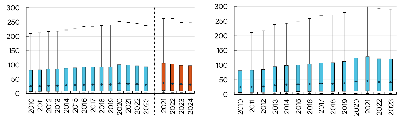
By this definition, approximately two out of three homeowners could increase their borrowing in 2023 (Chart 2.12, left panel).25 Among those homeowners, around half had a potential liquidity buffer equal to more than double their after-tax income (Chart 2.12, right panel). This share has increased over time, measured relative to after-tax income, but declined somewhat through 2023.
Share of homeowners with available collateral (LTV below 60%) by age group. Percent / Available collateral in the home as a share of after-tax income (LTV below 60%). Percent

19 The data do not continue after 2023 as the figures from the Norwegian Tax Administration, which include 2024, have not been processed in the same way as the income and wealth statistics for households from Statistics Norway.
20 Period: 2010–2023.
Households where the main income earner is under 25, over 90, or self-employed are excluded. Households in the top percentile of net wealth are also excluded. The boxplots show the 10th, 25th, 50th, and 75th percentiles (marked, respectively, by the lowest horizontal line along the black vertical line, the bottom of the blue box, the diamond, the top of the blue box).
21 Period: 2010–2024.
Households where the main income earner is under 25, over 90, or self-employed are excluded. Households in the top percentile of net wealth are also excluded. The boxplots show the 10th, 25th, 50th, 75th, and 90th percentiles (marked, respectively, by the lowest horizontal line along the black vertical line, the bottom of the blue box, the diamond, the top of the blue box, and the top vertical line along the black line).
The orange bars are estimates generated from tax assessments based on household composition from the previous year.
Liquid assets are defined as bank deposits, equity savings accounts and funds.
22 The data do not continue after 2023 as the figures from the Norwegian Tax Administration, which include 2024, have not been processed in the same way as the income and wealth statistics for households from Statistics Norway.
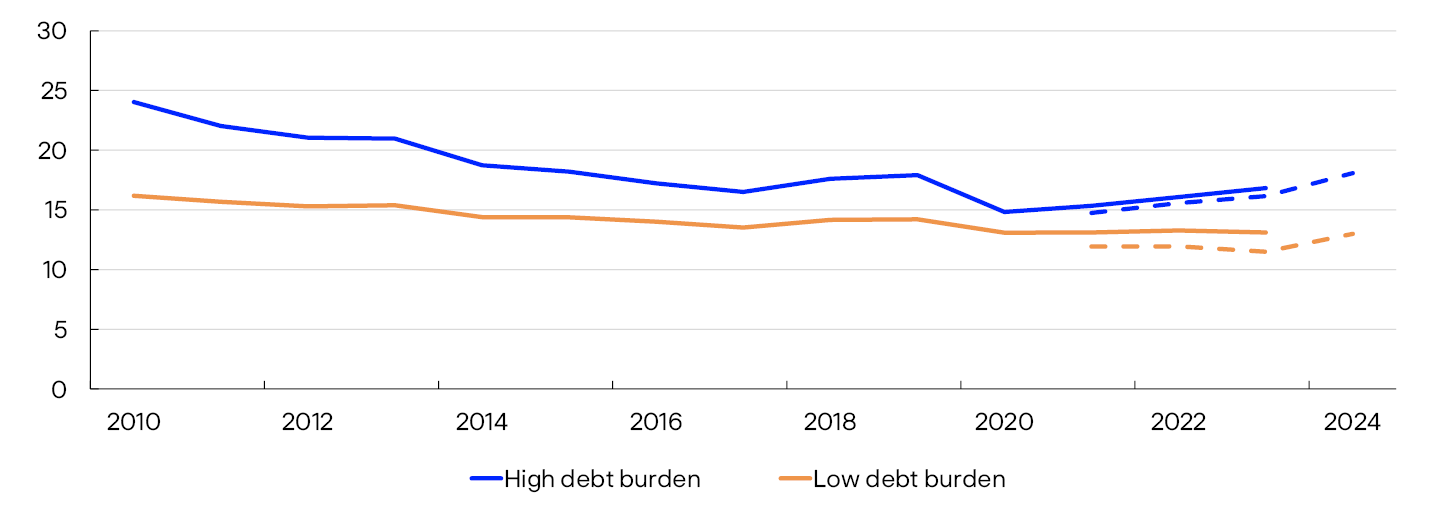
23 Period: 2010–2024.
Debt burden is debt as a share of after-tax income. Low debt burden is a debt burden below 300%. High debt burden is a debt burden above 300%. Households where the main income earner is under 25, over 90, or self-employed are excluded. Households in the top percentile of net wealth are also excluded. The dashed lines show figures from tax assessments and are estimates based on household composition from the previous year.
24 In such a situation, most households can relatively quickly and easily increase their mortgage up to an LTV ratio of 60%. Many can borrow more, but this is a limit that makes borrowing swiftly and easily available, making it a better measure of household ability to improve current liquidity. The Lending Regulations also have a maximum LTV ratio of 60% for home equity lines of credit.
25 The data do not continue after 2023 as the figures from the Norwegian Tax Administration, which include 2024, have not been processed in the same way as the income and wealth statistics for households from Statistics Norway.
26 Period: 2010–2023.
Available collateral is defined as households with a loan-to-value ratio below 60%. Loan-to-value ratio is defined as total debt minus student debt and unsecured debt as a share of the value of the primary residence. Households where the main income earner is under 25, over 90, or self-employed are excluded. Households in the top percentile of net wealth are also excluded. The boxplots show the 10th, 25th, 50th, 75th, and 90th percentiles (marked by, respectively, the lowest horizontal line along the black vertical line, the bottom of the blue box, the diamond, the top of the blue box, and the top vertical line along the black line).
2.4 Low residential construction and high demand contribute to higher house prices
The housing market is key to the assessment of financial stability, partly due to the interplay between house prices and debt.27 Homes are important assets for households and a key factor why they take on large debts. House prices have periodically risen considerably faster than household income, for example before the banking crisis in the early 1990s, before the financial crisis in 2008 and during the pandemic. This increased household sector vulnerability as household DTI ratios increased at the same time (Chart 2.1). In recent years, house prices as a share of disposable income have levelled off.
In 2024, prices in the secondary housing market increased by 3%. In the first half of 2025, house prices increased considerably. Regulatory easing of equity requirements for house purchases and expectations of lower interest rates may have contributed to the increase. However, house price inflation has since been lower. Looking ahead, house prices are expected to increase somewhat faster than household income due to lower interest rates and a low supply of new homes (see Monetary Policy Report 3/2025).
Lower housing affordability for households
When house prices increase faster than income over time, this may lead to fewer households gaining the opportunity to buy their own home. Such developments may influence households’ total borrowing and the distribution of risk between households, banks and other market participants. For banks, fewer new homeowners may dampen lending growth and reduce default risk if the most vulnerable households postpone buying a home to save more equity and benefit from higher income.
In connection with this Report, three analyses have been performed which shed light on developments in households’ access to the housing market and the behaviour of first-time buyers (see “Lower housing affordability in urban areas: how do first-time buyers respond?”). The first analysis indicates that housing affordability, defined here as the share of homes an individual can afford to buy with their own income within the debt-to-income requirements of the Lending Regulations, has declined over time, in particular in areas where housing demand is high. The other analysis finds that individuals with low income and/or low parental wealth postpone home purchases or remain longer in the rental market than before. The third analysis indicates that first-time buyers in the Oslo region, which is the area with the largest decline in housing affordability, to some extent postpone their purchase of a home until later in the life cycle and save more prior to purchase. They also receive more help to raise equity for home purchases than before, and the median size of the homes they purchase has changed little.
If access to homeownership is increasingly determined by parental wealth, the result over time could be a more uneven distribution of home ownership. On the one hand, such developments could strengthen households’ financial positions when they enter the housing market owing to higher equity levels. On the other, lower housing affordability can transfer more financing needs and risk on to the rental market, parents and other private financing sources or to new housing finance models, such as shared ownership and rent-to-own. If parents increasingly use accumulated equity to help their children enter the housing market, in isolation this may increase parents’ vulnerability to economic shocks if they therefore have smaller buffers to draw on. On the whole, the implications for financial stability are not clear.
Household formation is outpacing residential construction, particularly in urban areas
House prices are determined by a number of factors, including interest rates, income and tax policy stance. In addition, the supply of houses is a key driver of house prices over time. The relationship between the increase in the number of homes and the number of households is an indicator of developments in housing market supply and demand. In recent years, residential construction activity has been lower than household formation (Chart 2.13). The number of building permits and new home completions have fallen since 2022, partly driven by higher interest rates and increased construction costs. The number of building permits fell to very low levels in 2024, with the largest decline from 2022 in the counties of Telemark, Akershus and Innlandet. In the first half of 2025, the number of building permits increased somewhat compared with the same period in 2024.
Number of housing starts and completions and annual change in number of households. Thousands
The extent to which household formation has outpaced residential construction growth varies across regions (Chart 2.14). In the period between 2021 and 2024, household formation outpaced residential construction growth in all urbanisation classes, and over time, the difference is most marked in the main urban areas, which may have contributed to higher house prices in these areas.
Growth in the number of homes and households by urbanisation class. Percent
There are prospects for a pick-up in residential construction ahead
(see Monetary Policy Report 3/2025). Low supply of new homes and higher real household disposable income are expected to push up prices in the secondary housing market, which may boost the profitability of building new homes and contribute to more projects being realised. See Section 3.2 for a more detailed description of profitability and activity among real estate developers.
About underlying data for the analyses in this section
Analyses of households are based on statistics that use tax returns as the most important data source. Tax returns contain, inter alia, information about income, debt and wealth at the individual household level.
For the period to end-2023, complete income and wealth statistics for Norwegian households are used from Statistics Norway. For 2024, data are used from tax assessments from the Norwegian Tax Administration as at 8 August 2025. As tax returns do not include information on individuals’ household status, the previous year’s data on household composition from Statistics Norway’s income and wealth statistics are used to aggregate the variables up to household level.
27 Residential mortgage loans account for most household debt. Higher house prices raise the value of collateral and thus increase household borrowing opportunities. Higher house prices may result in increased credit demand over time, and improved access to credit may result in higher house prices through increased housing demand.
28 Period: 1990 – 2024.
A building permit is issued by the municipality allowing a developer to start construction. The permit is valid for 3 years.
A completed home is a building that has either been granted a temporary certificate of occupancy or a completion certificate, or a completed building exempt from permit requirements but still subject to notification and registration in the Cadastre.
A private household consists of people living in the same private dwelling. Statistics Norway (SSB) constructs private households based on information from the 2001 Population and Housing Census, which is continuously updated with data from the National Population Register, the Cadastre, and the Central Coordinating Register for Legal Entities.
29 Period: 2008 – 2024.
The charts use Statistics Norway’s urbanisation classes, which assign each municipality a value based on its urbanisation. The index is based on access to jobs and services, where a higher class indicates a less urban municipality.
A private household consists of people living in the same private dwelling. Statistics Norway (SSB) constructs private households based on information from the 2001 Population and Housing Census, which is continuously updated with data from the National Population Register, the Cadastre, and the Central Coordinating Register for Legal Entities.
Lower housing affordability in urban areas: how do first-time buyers respond?
When house prices rise faster than income, access to the housing market may change. In such situations, households can respond in multiple ways. Some remain longer in the rental market or live longer with their parents. Others receive significant financial transfers from their parents or other family members. A third response is to choose a more affordable home for example with a smaller area or in a more peripheral location. This box explores how availability in the housing market has changed and the responses made by first-time buyers to a sharp increase in house prices.
Housing affordability has fallen over time, especially in high-demand housing areas
In a recent analysis from Norges Bank, housing affordability, here defined as the share of homes that an individual has the means to purchase based on own income, is calculated in 2023 compared with 2013.1
The analysis indicates that housing affordability fell considerably in Oslo during this period, has fallen somewhat in urban areas excluding Oslo and otherwise remained reasonably stable in the rest of Norway (Chart 2.A). In Oslo, the share of homes that individuals with median incomes can afford has fallen from 15% in 2013 to 5% in 2023. In other urban areas, the share fell from 25% to 19%. This indicates a widening gap between income and house prices in the most urban areas.
Share of homes that can be purchased for five times gross income across the income distribution

Low income and low parental wealth is increasingly linked with later home purchases
In another analysis from Norges Bank, persons born between 1985 and 1991 are followed from the age of 20 until their first home purchase.3 Each cohort is divided into income brackets based on the year they turn 30 and based on their parents’ financial wealth in the year before they turn 20. We find that the share of individuals that have purchased their own home by the age of 32 is higher the higher their income and the larger the wealth of their parents is (Chart 2.B, left panel). The share of individuals that have purchased a home increases in particular for those with low or medium income, the increase is significant for individuals with higher parental wealth. For individuals with high income, more than 80% have purchased a home by the age of 32, independent of parental wealth. By comparison, for individuals with low income and low parental wealth, only around 25% have purchased a home by the age of 32. This share increases to around 45% if parental wealth is high.4
Share owning a home by the age of 32. 1991 cohort / Change from the 1985 to the 1991 cohort in the share owning a home at the age of 32

These differences are more significant for the younger age cohorts in the dataset. Compared with the 1985 cohort, the percentage of individuals who have purchased a home by the age of 32 is lower for the 1991 cohort, particularly among those with low income and/or low parental wealth (Chart 2.B, right panel).6 This indicates that a higher number of individuals with relatively low income, low parental wealth or both postpone a home purchase or remain in the rental market. The findings are consistent with patterns observed in other studies of first-time buyers in Norway and the Nordic region. These studies show that financial support from family members has gained more importance at the household formation stage.7
First-time buyers in the Oslo region save more before buying a home
In a third analysis, we look at the extent to which young households resident in the Oslo region, and who purchased their first home in the region in the period 2011–2023, have responded to higher house prices.8 Unlike in the two analyses above, homebuyers here are grouped annually by estimated maximum purchase price based on income in the year of purchase, as well as by wealth and debt at the end of the preceding year.9
We find that first-time buyers in the Oslo region to some extent postpone the purchase of a home to later in the life cycle, as found in the analysis described above. This is shown by a declining share of households under the age of 25 that buy a home, whereas the share of households between 26 and 30 has increased (Chart 2.C, left panel).10 This result likely reflects that first-time buyers save more equity prior to a home purchase. In line with this, first-time buyers have increased their financial wealth over time (Chart 2.C, right panel).
The share of households purchasing a home at different ages. Percent / Financial wealth at the the end of the year prior to purchasing a home, as a share of income. Percent
At the same time, we find that the change in equity from the preceding year to the year following households’ first-time home purchase has increased over the period, and the most for those with a low maximum purchase price (Chart 2.D, left panel). This implies that first-time buyers to a larger extent than before receive parental financial support to establish initial equity, likely through family transfers.12 We find that the size of the home has changed relatively little over time, but there are some signs of downsizing (Chart 2.D, right panel)13. The figures also show that first-time buyers purchase approximately homes of the same size independent of the estimated maximum purchase price. This implies that there may be factors other than the maximum purchase price that determine the size of the home purchased, for example household size. Furthermore, the relatively modest reduction in house size reflects the relatively limited scope of homes to choose from in the limited region in this study for the majority of first-time buyers and the limited possibilities to downsize.14
Median change in equity from the year before to the year after a home purchase. In millions of 2024 NOK / Median square meters

1 See B. H. Vatne (2025) “Kjøpekraften i boligmarkedet har falt” [Affordability in the housing market has fallen]. Blog post published on the Bankplassen blogg. Norges Bank. (in Norwegian only). The analysis shows that maximum household borrowing is five times gross income, the same as the maximum DTI ratio set out in the Lending Regulations.
2 Period: 2013 – 2023. The sample consists of individuals aged 20–35 with employment income above the basic amount of the National Insurance Scheme (G) for both years. The Oslo region comprises the municipalities of Oslo, Bærum, Asker, Lillestrøm, Nordre Follo, Ullensaker, Nesodden, Ås, Lørenskog, and Nittedal. Other urban areas are Stavanger, Sandnes, Sola, Moss, Sarpsborg, Fredrikstad, Frogn, Vestby, Rælingen, Gjerdrum, Drammen, Lier, Hamar, Horten, Tønsberg, Bergen, and Trondheim
3 See Solheim, H., and B. H. Vatne (2025) “Endringer i andel boligkjøpere i Norge fra 1985-kohorten til 1991-kohorten: Forskjellene har økt”. [Changes in home-purchase likelihood in Norway between the 1985 cohort and the 1991 cohort: the differences have widened]. Staff Memo 11/2025. Norges Bank. (in Norwegian only).
4 The chart shows the result for the 1991 cohort, but the finding also applies to the other cohorts.
5 Income group is defined based on an individual’s income at age 30. High income is defined as the 20% highest earners, while low income is defined as the 20% lowest earners. Medium income is defined as the median income. Parental wealth is defined based on parents’ liquid wealth the year before the individual turns 20. Liquid wealth is the sum of bank deposits and holdings in investment funds. High parental wealth is defined as the 20% with highest liquid parental wealth, while low wealth is defined as the 20% with lowest liquid parental wealth. Medium parental wealth is defined as the median.
6 In the analysis, a regression analysis has also been performed that confirms this result when we control for developments in, for example, expected income, parental wealth, education and residence over time.
7 See eg Omholt E. L. (2025) “Unge uten formuende foreldre eier sjeldnere bolig, særlig i Oslo” [Young people without wealthy parents own homes less frequently, particularly in Oslo]. Statistics Norway. (in Norwegian only).
8 See Ellingsen, J., P. Nenov, H. Solheim and B. H. Vatne (2025) “The evolution of first-time buyers in the Oslo region”. Staff Memo 10/2025. Norges Bank.
9 We calculate the maximum purchase price based on households meeting the requirements of the Lending Regulations, according to the version of the Regulations at year-end 2024. The maximum LTV ratio was the binding requirement for the majority of households in the sample studied here.
10 The broad-based decrease in 2023 reflects the sharp increase in interest rates and inflation.
11 Period: 2011–2023. The sample comprises households with the main income earner aged between 20 and 35 who purchased their first home in the respective year. The deciles of maximum budget are calculated based on the maximum amount the household can afford to pay for a home, provided they also meet the following criteria:
1) The loan cannot exceed 85% of the home’s value
2) Total debt cannot exceed 5 times gross income
3) The household must have sufficient after-tax income to cover normal expenses in the event of a 3 percentage point interest rate increase (but at least 7%)
12 Figures from Statistics Norway’s survey on housing conditions show that one in four homebuyers in the period 2019–2023 received parental financial support to purchase a home, see Statistics Norway (2025) “Housing conditions, survey on living conditions. StatBank source table 14075: Purchase of dwellings, by income group. Individuals 2012–2023.”. Figures from the Norwegian Association of Real Estate Agents show that 67% of young homebuyers in Oslo received parental financial assistance in 2023, see the Norwegian Association of Real Estate Agents (2025) “Førstegangskjøpere 2025 Q2” [First-time buyers 2025 Q2) (in Norwegian only). Furthermore, a study from Norges Bank shows that households with more affluent parents have an almost 15% higher likelihood of becoming homeowners by the age of 30, see Wold, E. G., K. A. Aastveit, E. E. Brandsaas, R. E. Juelsrud and G. J Natvik (2023) “The housing channel of intergenerational wealth persistence”. Working Paper 16/2023. Norges Bank.
13 The chart shows the median, but the result also applies when analysing other parts of the distribution.
14 One possible response not reflected in this analysis is households moving out of the region.
15 Period: 2011–2023. The sample comprises households with the main income earner aged between 20 and 35 years old who purchased their first home in the respective year. The deciles of maximum budget are calculated based on the maximum amount the household can afford to pay for a home, provided they simultaneously meet the following criteria:
1) The loan cannot exceed 85% of the home’s value
2) Total debt cannot exceed 5 times gross income
3) The household must have sufficient after-tax income to cover normal expenses in the event of a 3 percentage point interest rate increase (but at least 7%)
Housing-related costs may increase due to more frequent extreme weather events
Weather patterns and the climate in Norway are changing. Average temperatures have risen, and precipitation is more often intense, increasing the cost and frequency of building damage. Claims payments from Norwegian non-life insurance companies have increased markedly in recent decades (Chart 2.E), both for natural disasters (floods, avalanches, landslides, storms and storm surges) and damage resulting from stormwater intrusion.
Payouts. In millions of 2024 NOK. 2008-2024
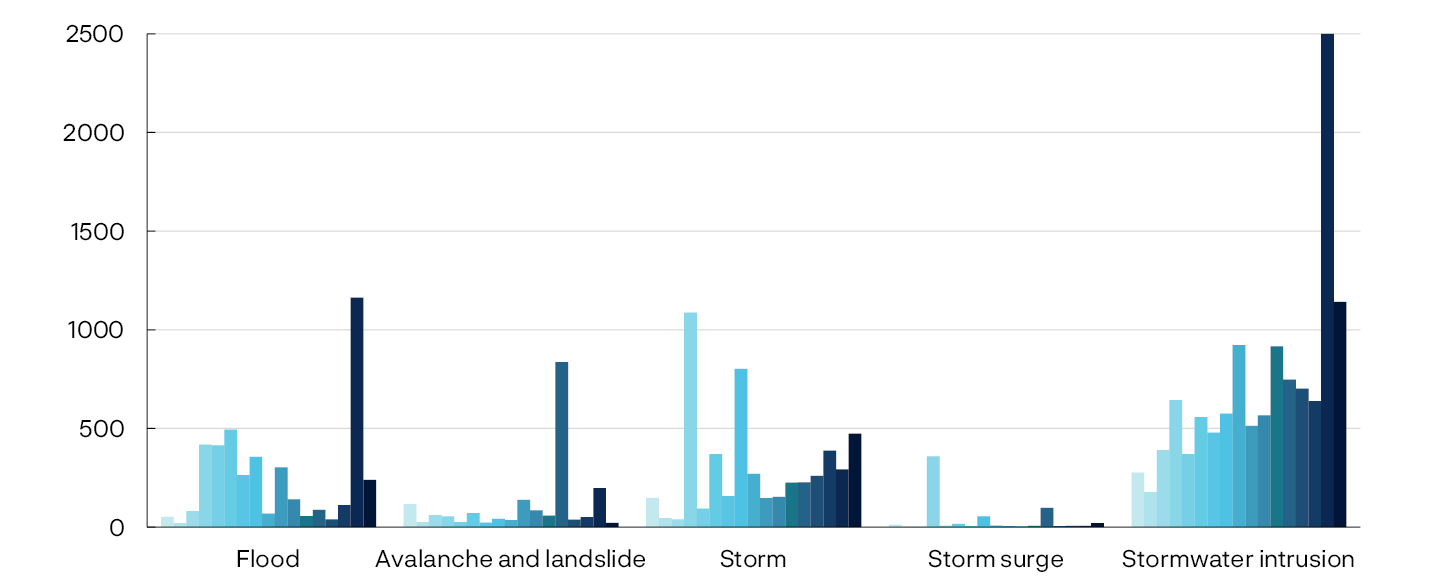
At present, there is reason to believe that access to insurance and insurance coverage in Norway are sufficient.2 In comparison, insurance coverage in a number of European countries is low, and in some regions in the US, access to insurance and credit has become limited in areas at high risk of natural disasters. Norwegian insurance policy holders are covered against natural disasters through their fire insurance policy, which includes mandatory membership in the Norwegian Natural Perils Pool. Stormwater intrusion damage, however, is covered by regular private home insurance. Premiums and deductibles normally increase in response to rising damage costs, and insurance policy terms and conditions may become more stringent. This may reduce Norwegian households’ insurance coverage. In addition, homeowners have to take into account that even though a significant share of damage costs is covered by the insurance company, there is always a risk that more frequent weather events may reduce house prices and have a localised negative impact on economic activity and wage developments.3
Following the extreme weather event “Hans”, the rise in home insurance premiums has outpaced CPI inflation in recent years, particularly from 2023 to 2024 (Chart 2.F). In addition, after 2020, municipal fees have risen much faster than CPI inflation owing to wear and tear on public infrastructure. If changing weather patterns lead to rising municipal expenses and insurance payouts, with subsequent increases in municipal fees and insurance premiums, households’ housing-related costs can be expected to rise in the coming years.
4Average cost of municipal fees and home insurance
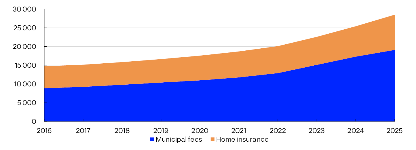
In addition to large differences in risk between individual homes, there are systematic differences between different types of homes. Figures from 7Analytics that Norges Bank has accessed indicate that detached and semi-detached houses are more exposed to stormwater intrusion than flats, and the share of high-risk homes is somewhat higher in Northern and North-Western Norway (Chart 2.G).5 The share of loans secured on vulnerable detached and semi-detached houses also differs across banks (Chart 2.H).
Average index values for stormwater exposure across counties. Distribution of stormwater index across building types
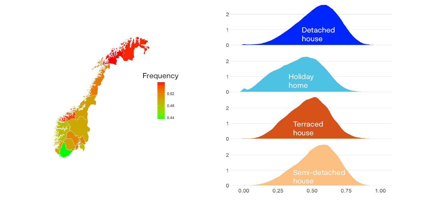
Share of property value pledged to banks as collateral with elevated stormwater risk
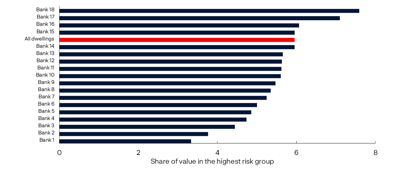
Damage caused by more extreme weather events can be mitigated by measures such as improved water management and changes in building materials and design. To ensure sound risk management, adequate mapping of risk factors will be important. A clearer overview of such factors is provided from, for example, publicly available maps (Norwegian Mapping Authority, Norwegian Water Resources and Energy Directorate and Norwegian Centre for Climate Services) and new risk indicators developed by insurance companies and technology clusters (such as 7Analytics). Such mapping may result in clearer insurance policy terms and conditions (relating to drainage requirements for example) and targeted mitigation measures.
Improved mapping of risk profiles may provide insurance companies with a basis for formulating clearer insurance policy terms and conditions, such as drainage requirements and other mitigation measures to maintain insurance coverage. Insurance companies can also use such mapping to increase the degree of premium differentiation when determining risk. At the same time, informed collaboration between insurance companies, municipalities and homeowners may lead to more mitigation efforts and improved cost control over time.
Overall, developments indicate that Norwegian homeowners must be prepared for somewhat higher housing-related costs related to physical climate risk. Sound information, mitigation measures and clearer regulation may dampen costs and strengthen resilience among households and in the financial system.
1 Period: 2008-2024.
The chart shows annual insurance payouts as reported by Finance Norway for five different types of weather-related damages: floods, avalanches and landslides, storms, storm surges and stormwater intrusion. The amounts are in constant 2024 NOK. The chart shows that payouts have increased markedly from 2008 to 2024. For floods and stormwater intrusion, there was a particularly high peak in 2023 during the storm “Hans”.
2 Note that there is no publicly accessible database showing which homes have home insurance. As reported by Finance Norway, insurance companies had insured slightly more than 1.4 million detached and semi-detached houses in 2025 H2. According to Statistics Norway, there are slightly more than 1.8 million such houses in Norway.
3 See Espegren, C., M. E. Garcia-Appendini, S. M. Galaasen and M. Mæhlum (2025): “Weathering the storm: The effects of Natural Disasters on Households under Universal Insurance”, unpublished manuscript.
4 Period: 2016–2025. The chart shows the average expenses for a detached house related to municipal fees and home insurance in constant 2024 NOK. The chart implies that the cost has increased from about NOK 15 000 in 2016 to NOK 30 000 in 2025. Both municipal fees and home insurance expenses have increased.
5 See Solheim, H. and B. H. Vatne (2025) “Skader forårsaket av endringer i vær og klima: Kartlegging av norske boliger i risikosoner for værrelatert risiks” [Damage caused by weather and climate change: Potential risk to Norwegian homeowners]. Staff Memo 12/2025. Norges Bank. (In Norwegian only.)
6 The chart shows the distribution of index values for the risk of stormwater damage as estimated by 7analytics. The index measures the likelihood that a home could be damaged by stormwater given heavy rainfall, and ranges from 0 (not likely) to 1 (very likely). The left panel shows the average value across counties. The counties in Northern Norway, Møre og Romsdal, and Buskerud have the highest values. The right panel shows the distribution of index values for four types of residential buildings: detached house, holiday home, terraced house, and semi-detached house. Detached houses and semi-detached houses have a higher average index value and a larger share of high index values.
7 The chart shows the share of values pledged to the banks as collateral of detached and semi-detached house with elevated stormwater risk. Eighteen Norwegian banks. The chart shows significant differences in exposure to high-risk homes across banks, but a majority of banks are less exposed than Norway as a whole. All dwellings also include unmortgaged homes.
Households with high debt-to-income ratios have reduced consumption the most in response to higher interest rates
In the years 2020 to 2023, there were wide fluctuations in overall household consumption (Chart 2.I). In 2020, the first year of the pandemic, saving increased markedly and consumption fell substantially despite the widespread increase in household income. In the years that followed, consumption increased significantly, primarily due to lower saving, while in 2023 higher interest rates and high inflation led to lower consumption. The sharpest decline in consumption owing to higher interest rates was among households with high debt-to-income (DTI) ratios, while households with bank deposits and little to no debt were more resilient.
Change in consumption per household. Constant prices. Percent
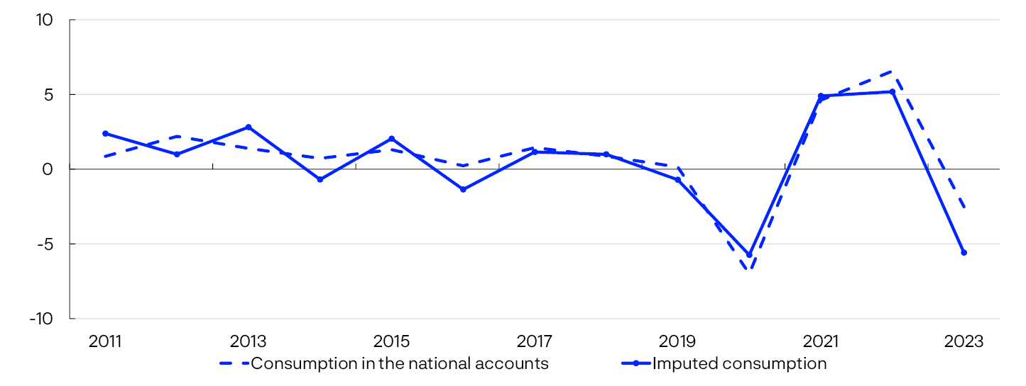
To better understand the fluctuations in consumption in this period, Norges Bank has conducted a recent analysis that seeks to estimate consumption per household.2 As direct consumption data are not available in public databases, household budget constraints are used as a basis to derive imputed consumption as the difference between income and saving. This estimated level of household consumption corresponds well to total household consumption in the national accounts.
To shed light on the differences in consumption, households are grouped by DTI ratio into three tertiles (Chart 2.J).3 The group with low DTI ratios includes households with no debt. The group with high DTI ratios has an average ratio close to 3. The chart shows substantial differences between the groups in both consumption developments and the change in contributions from different income items, such as interest expenses and wage income. In 2021, for example, consumption increased the most among households with high DTI ratios, driven primarily by income growth, lower interest expenses and a drawdown of savings.
Decomposition of change in consumption. In thousands of 2015 NOK

In 2023, consumption fell in all the household groups, but the most among households with high DTI ratios. Higher interest expenses dampened disposable income substantially for this group. Real wage income fell in all the household groups, but the least among households with high DTI ratios. This is likely due to households with a high DTI ratio often having higher wage growth. When controlled for other factors that may influence the relationship between changes in consumption and DTI ratios, such as liquid buffers, there is still a clear correlation between DTI ratios and consumption cutbacks, and the results indicate that households with low liquidity buffers reduce consumption the most.5
1 Period: 2011–2023.
2 See Guldbrandsen, M. A. H., S. L. Nilsen and E. S. Njølstad (2025) “Revisiting imputed consumption expenditure during the recent tightening cycle in Norway”. Staff Memo 13/2025. Norges Bank.
3 Group 1 comprises households with DTI ratios between 0 and 0.32. Group 2 comprises households with DTI ratios from 0.32 to 2.14. Group 3 comprises households with DTI ratios above 2.14.
4 Period: 2019–2023. Debt ratio is defined as household debt relative to total pre-tax income.
Households are divided into 3 tertials based on their DTI ratio in the previous year.
5 The control variables in the model are the level of consumption and gross wealth in 2022, change in after-tax income, age and household composition. The correlation between a change in consumption and DTI ratios is also negative and significant if we measure the change in consumption as a percentage. See Guldbrandsen, Nilsen and Njølstad (2025) “Revisiting imputed consumption expenditure during the recent tightening cycle in Norway”. Staff Memo 13/2025. Norges Bank.
Households cut consumption when house prices fall, but the isolated effect is moderate
Experiences from global crises such as the US during the financial crisis, show that a combination of high indebtedness and a fall in house prices may lead to a severe downturn, both directly through bank losses and indirectly through weakened consumption.1 Recent research often finds weaker links than earlier studies.2 A new analysis from Norges Bank uses the fall in oil prices in 2014–2015, which particularly affected the Stavanger region, as the basis for understanding how a local fall in house prices affects household consumption without a simultaneous effect from national or international unrest, and for understanding which spillovers such a consumption change has on the local economy.3 4The fall in oil prices led to a sharp fall in house prices in Stavanger, but the rest of Norway was unaffected (Chart 2.K).
House prices in Stavanger and surrounding areas and in the rest of Norway. 2014 Q4 = 100
In the analysis, we compare changes in consumption expenditure of public sector workers in Stavanger – who experienced a fall in house prices but had stable incomes through the period – with equivalent groups in the rest of Norway. In this way, we seek to isolate the effect of a fall in house prices from changes in income. The analysis is conducted using card transaction data on an individual level, which allows us to measure consumption response to a fall in house prices more precisely than with macro variables.6
The results indicate that households reduce consumption expenditure when house prices fall (Chart 2.L). Households reduce consumption expenditure on average by 3.5% of the fall in house prices, distributed over three years. A fall in house prices of NOK 500 000 corresponds to a reduction in consumption expenditure by NOK 500 per month. These results are in line with findings in more recent international studies.7 At the same time, there is reason to believe that the effect is dependent on the size of the fall in house prices, and that the reduction in consumption expenditure is relatively larger in response to a steeper fall in house prices.
Estimated consumption response as a share of a fall in house prices
The analysis also shows that the effect is markedly stronger for households with high DTI ratios.9 The effect is most pronounced for credit-limited households, here defined as those with debt amounting to more than four times annual income or with loan-to-value (LTV) ratios of more than 90%.10 These households cannot take on more debt unless income or home values increase significantly. Corresponding differences between households with lower levels of debt are not observed.
Reductions in consumption expenditure among credit-constrained households primarily affect durable consumer goods such as those used for renovation, furniture and other major purchases (Chart 2.M). Households with lower DTI ratios also reduce expenditure on such consumer goods, but considerably less. Among other goods, the differences between the two groups are smaller. The analysis also shows that the rise in households’ borrowing declines following a fall in house prices. This implies that it is more difficult for highly indebted households to refinance debt when house prices fall and that they therefore postpone costly renovation projects.
Change in consumption of different types of goods for households with high and low debt ratios
Overall, this analysis provides a more nuanced picture of how a fall in house prices influences consumption expenditure than earlier studies from the US. At the same time, the fall in house prices in Stavanger was less pronounced than in the US during the financial crisis and consumption expenditure is likely to be reduced relatively more if there are steeper falls in house prices. Consumption expenditure will also be reduced more if the fall in house prices occurs together with other negative shocks, for example if there is high unemployment. At the same time, institutional frameworks and social safety nets are also likely to dampen the impact in Norway.
1 See Mian, A., K. Rao og A. Sufi (2013) “Household balance sheets, consumption, and the economic slump”. The Quarterly Journal of Economics, 128 (4), pp 1687–1726 and Dynan, K., A. Mian and K.M. Spence (2012) “Is a household debt overhang holding back consumption?”. Brookings Papers on Economic Activity, pp 299–362.
2 See eg Aladangady, A. (2017) “Housing wealth and consumption: Evidence from geographically-linked microdata”. American Economic Review, 107(11), pp 3415–3446, Andersen, H. Y. and S. Leth-Petersen (2021) “Housing wealth or collateral: How home value shocks drive home equity extraction and spending”. Journal of the European Economic Association, 19(1), pp 403–440 and Gulbrandsen, M. A. H. (2023) “Does high debt make households more vulnerable? A survey of empirical literature using microdata”. Staff Memo 3/2023. Norges Bank.
3 See Aastveit, K. A., Böjeryd, J., Gulbrandsen M. A. H., Juelsrud, R. E., and Roszbach, K. (2025) “What Do 12 Billion Card Transactions Say About House Prices and Consumption?” Working Paper 15/2025. Norges Bank.
4 Earlier studies based on Norwegian microdata include Fagereng, A. and E. Halvorsen (2016) “Debt and household consumption responses”. Staff Memo 1/2016, Norges Bank and Fagereng, A., G. J. Natvik, and J. Yao “Housing, Debt, and the Marginal Propensity to Consume”. Unpublished manuscript. These studies do not directly examine a fall in house prices, but find some support for a fall in consumption if wealth decreases and that the response from credit-constrained households is likely to be more pronounced. A study based on data at a regional level in Norway finds that a fall of 10% in house prices correlates to a reduction in car and retail sales of 2%, see Grindaker, M. H. (2017) “House prices and households’ consumption”. Staff memo 11/2017, Norges Bank.
5 Period: 2011 Q1 – 2017 Q4.
The chart shows the house price index for the Stavanger area and the average index for the rest of Norway. Both are indexed to 100 in 2014 Q4. The regions are defined by Real Estate Norway.
6 See Aastveit, K. A., Böjeryd, J., Gulbrandsen M. A. H., Juelsrud, R. E., and Roszbach, K. (2025) “What Do 12 Billion Card Transactions Say About House Prices and Consumption?” Working Paper 15/2025. Norges Bank.
7 See eg Aladangady, A. (2017) “Housing wealth and consumption: Evidence from geographically-linked microdata”. American Economic Review, 107(11), pp 3415–3446.
8 Period: 2012 Q1 – 2018 Q4.
The chart shows the estimated marginal propensity to consume in response to a fall in house prices. The solid blue line shows the point estimates, and the dashed blue lines show the 95% confidence interval. The dark vertical dashed line is at 2014 Q4, when house prices in the Stavanger area began to fall. Each individual point shows the consumption response at that point in time, relative to the total fall in house prices over the period from 2014 Q4 to 2018 Q4. Estimated using an instrumental variable regression. For more details, see Aastveit, K. A., Böjeryd, J., Gulbrandsen M. A. H., Juelsrud, R. E., and Roszbach, K. (2025) “What Do 12 Billion Card Transactions Say About House Prices and Consumption?” Working Paper 15/2025. Norges Bank.
9 See Aastveit, K. A., Böjeryd, J., Gulbrandsen M. A. H., Juelsrud, R. E., and Roszbach, K. (2025): “What Do 12 Billion Card Transactions Say About House Prices and Consumption?” Working Paper 15/2025. Norges Bank.
10 The thresholds in the analysis of 90% and four times annual income, respectively, are set so that homeowners will likely be able to increase LTV ratios if they are within the thresholds. The current Lending Regulations have a limit for the maximum LTV ratio of 90% of the home value and a maximum DTI ratio of five times gross income. Over the time period examined by the analysis, the requirements were worded slightly differently.
11 The chart shows estimated marginal propensity to consume for different categories of goods in response to a fall in house prices as of 2017 Q4. Circles show point estimates and lines show the 95% confidence interval. Red points and lines show the response for households with a debt ratio above 4. Black points and lines show the response for households with a debt ratio below 4.
3.1 Norwegian firms are solid overall
Financial positions in the Norwegian corporate sector were stable through 2024 after having weakened somewhat in pace with higher interest rates in the two preceding years.1 Annual financial reporting shows that corporate sector solvency had improved and that profitability2 was marginally weaker than in 2023. The outlook is also stable. According to Regional Network contacts, output growth increased somewhat in early 2025, and contacts expect growth to remain elevated through 2025 H2, see Regional Network 3/2025.
Corporate sector solvency improved in 2024 and is strong overall. Annual financial statements show that equity ratios increased in most sectors, following a decline in several sectors in the two preceding years (Chart 3.1). Retained earnings, in particular, increased in 2024, ie firms retained a substantial share of profit for the year. Bank and bond debt growth was moderate through 2024.
Equity ratio. Percent
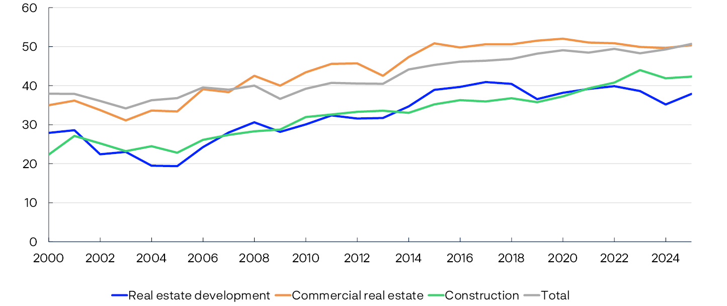
Profitability, as measured by firms’ operating margins, declined marginally in 2024 (Chart 3.2). For sectors with high debt-to-income ratios, such as real estate development and commercial real estate (CRE), interest expenses have reduced profitability considerably since 2022. In real estate development, operating margins after interest expenses were marginally higher than in 2023, but only barely higher than during the 2008 financial crisis. In spite of persistently low activity in the construction industry, profitability was broadly unchanged between 2023 and 2024 and not far from its historical average.
Operating margins before and after net interest expenses. Percent
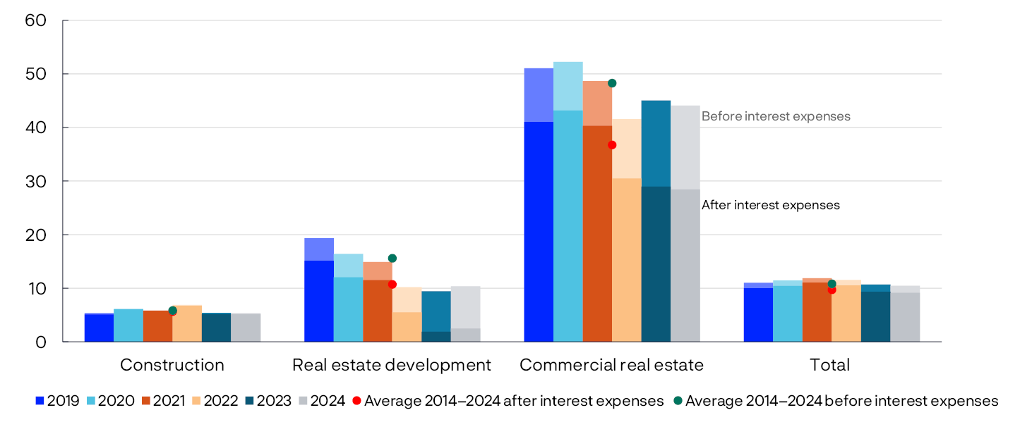
1 The financial statement analysis covers Norwegian non-financial limited companies that have submitted annual financial statements for the applicable year. Firms in oil and gas extraction and power companies are omitted from the analysis owing to substantial earnings volatility that has a disproportionately large impact on overall developments. Banks’ exposures to such firms are relatively small.
2 Measured as EBITDA/revenue and (EBITDA-net interest expenses)/revenue.
3 Period: 2000–2024.
Equity ratio is book equity as a share of total capital (equity and debt).
4 Period: 2019–2024.
Operating margins before interest expenses are earnings (EBITDA) as a share of turnover. Operating margins after interest expenses are earnings (EBITDA) minus interest expenses plus interest income, as a share of turnover.
Net interest expenses are shown by the shaded areas in the chart.
3.2 Direct effect of higher tariffs on Norwegian firms is likely limited
Earlier in 2025, US import tariffs were raised substantially. Higher tariffs will likely dampen global growth but so far do not appear to have affected the corporate sector in Norway or abroad to any great extent.5
Among Regional Network contacts that export directly to the US, some report concern that they will lose market shares to competitors in countries subject to lower tariffs (Regional Network 2/2025). Some suppliers, including firms in the metal industry, report weaker demand and link this to the increased supply of Asian products in the European market.6 However, most export-oriented firms expect sound growth in H2.
The tariffs could primarily lead to changes in which markets Norwegian firms export to. This applies in particular to the aquaculture sector as the US is one of the largest export markets for Norwegian farmed salmon. More traditional fisheries largely export to other markets. However, a broader global downturn may also have negative spillover effects for traditional fisheries.
Lending to fisheries and aquaculture accounts for about 6% of banks’ total Norwegian corporate exposures (Chart 3.3). However, there are large differences between banks, and for the most exposed banks, these two sectors account for more than 20% of corporate exposures. Overall, aquaculture accounts for close to 60% of these exposures. However, the ten banks with the highest exposure to fisheries and aquaculture are most exposed to fisheries.
Lending to fisheries and aquaculture as a share of total corporate exposure per bank. Percent
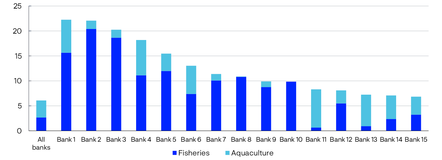
Aquaculture exports will likely be redirected to other markets
The export value of Norwegian farmed salmon has increased substantially in recent years, in particular due to a weak krone and high demand. At the same time, the aquaculture sector has long struggled with problems such as fish health and large fluctuations in operating costs. This has resulted in substantial volatility in the sector’s operating margins (Chart 3.4). However, the return on capital has been high over time.
The quantity of seafood produced by Norwegian firms is primarily determined by supply-side conditions. If US demand were to fall, exports could to a large extent be shifted to other markets. A number of aquaculture contacts in Norges Bank’s Regional Network expect that more farmed salmon from Chile and Canada, which have lower tariffs, will be exported to US markets, while Norwegian salmon will, to a greater extent, be directed at European and Asian markets. With fewer markets, salmon export prices may decline and weaken sector profitability somewhat.
The EU, the most important market for Norwegian seafood, has adopted tariff quotas for fish and aquaculture that entail reduced or no tariffs on several imported products. Although agreements with the EU provide relatively good market access, fish and aquaculture products are not fully integrated in the EEA Agreement for goods in general. Changes to tariff quotas may force Norwegian salmon to compete under different conditions in European markets, which may reduce demand and potentially further dampen export prices.8
On the other hand, Regional Network contacts report that improved fish health has contributed to substantial output growth in aquaculture in the first half of 2025, and contacts expect continued growth to the end 2025, see Regional Network 3/2025. Higher output as a result of improved fish health could help maintain profitability even if export prices decline.
Lower fishing quotas make fisheries vulnerable to price falls
In recent years, stocks have declined markedly for many species of fish,9 leading to gradual fishing quota cuts every year.10 However, profitability in the fisheries sector has been buoyed by a strong increase in fish prices, in particular for cod. Operating margins fell somewhat in 2022 and 2023 but increased somewhat again in 2024 (Chart 3.4).
Operating margins. Percent
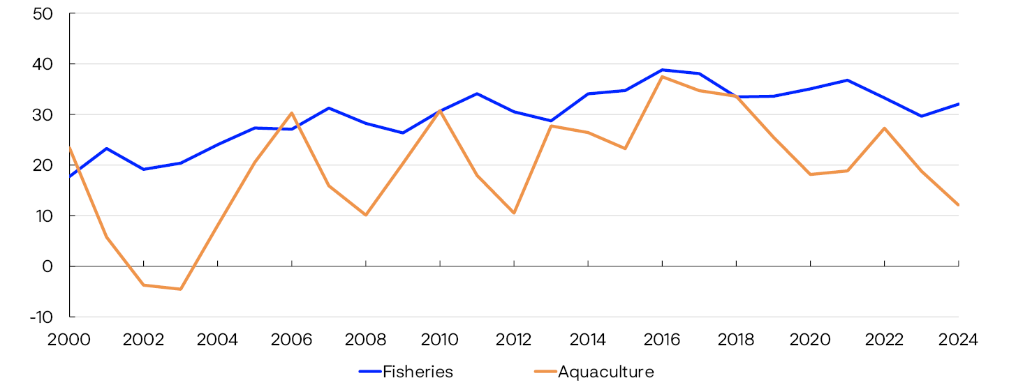
Lower quotas and high price sensitivity make fisheries vulnerable to a decline in export prices. A global downturn or more adverse trade policies could push down fish prices and reduce sector profitability considerably. This may result in higher credit risk and tighter credit supply from some banks with considerable exposure to fisheries (Chart 3.3).
There is still considerable uncertainty surrounding global developments
In the longer term, higher tariffs and persistent trade tensions could contribute to lower global growth and higher financial market uncertainty. A more protectionist trade system may dampen investment, disrupt global supply chains and weaken productivity growth, which overall may increase credit risk for banks with high exposure to export-oriented industries.12
5 International Monetary Fund (2025) “Shifting Ground beneath the Calm”. Global Financial Stability Report. IMF, October 2025, Section 1, subsection “Corporate Credit Risk—The Corporate Sector Is Resilient to Tariffs So Far”, p 29.
6 Banks’ exposures to the metal industry are negligible.
7 Figures as of 30 June 2025.
8 European Commission – Directorate-General for Trade (2025) “EU trade relations with Norway. Facts, figures and latest developments”. EU Trade website. European Commission (2025).
9 In particular for Northeast Arctic cod.
10 Overall, quotas have been reduced by around 50% since the peak in 2019–2020, see KPB and Oslo Economics (2025) “Kunnskapsgrunnlag – Effektene av fiskekvotereduksjoner i Nordland” [Basis – Effects of fish quota reductions in Nordland] (in Norwegian only), Nordland local government authority, August 2025.
11 Period: 2000–2024.
Operating margins are earnings (EBITDA) as a share of revenue.
12 International Monetary Fund (2025) “Global Economy in Flux: Prospects Remain Dim”. World Economic Outlook. IMF, October 2025.
3.3 Higher number of bankruptcies in real estate development
Weaker economic developments contributed to a gradual increase in the share of bankruptcies among Norwegian firms through 2023 and 2024. At the same time, the increase must be viewed in the context of a normalisation following unusually low bankruptcy figures during the pandemic. So far in 2025, the bankruptcy rate has been relatively stable and at approximately the same level as the average rate for the past ten years (Chart 3.5).
Share of firms that have gone bankrupt in the past 12 months. Percent
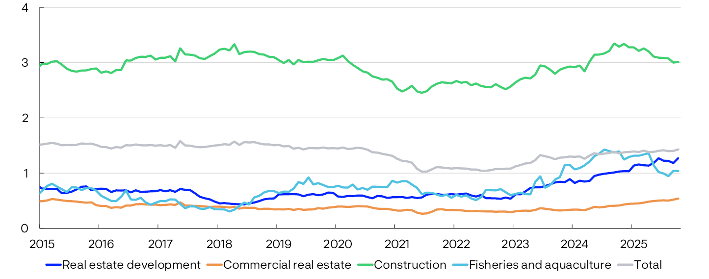
The share of bankruptcies in the fisheries and aquaculture sector increased through 2023 and 2024. The increase is primarily in fisheries and relates to higher financing costs and lower fishing quotas. So far in 2025, bankruptcies have declined somewhat. Bankruptcies in this sector have mostly affected smaller firms.
Bankruptcies in the real estate sector have increased in recent years, reflecting higher interest expenses and low construction activity, which have impacted this sector in particular. The share of bankruptcies in real estate development has risen sharply and is higher than during the financial crisis. Bank debt related to bankrupt real estate developers has increased substantially in recent years (Chart 3.6). So far in 2025, bank debt of bankrupt real estate developers amounts to NOK 1.8bn, around ten times the average in the years before bankruptcy figures started to rise. Large individual bankruptcies account for a considerable part of this bank debt. So far in 2025, bankruptcies in real estate development account for 21% of total bank debt in bankrupt firms, which is relatively high given the size of the sector. See Section 3.4 for a further discussion of the real estate development market.
Total bank debt of real estate developers that have gone bankrupt. In billions of NOK
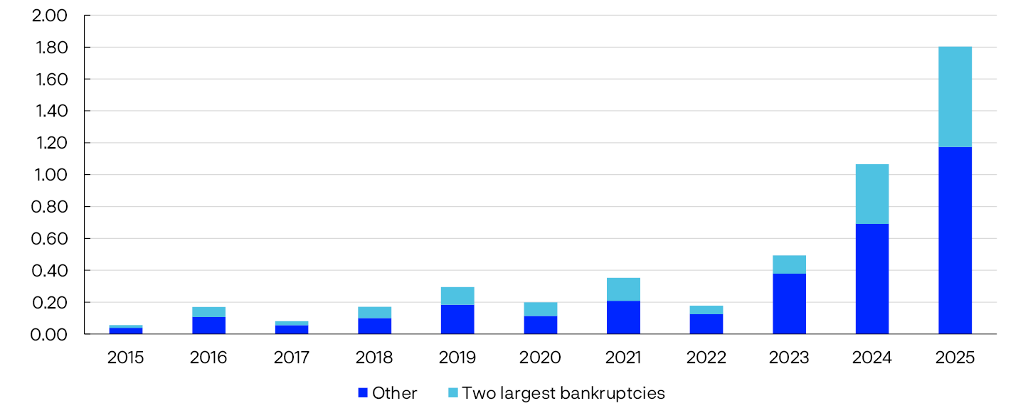
The number of bankruptcies has also risen in commercial real estate, but to a lesser extent. Higher bankruptcy rates are normal in the construction industry as building contractors often have small margins and low capitalisation, which makes them more vulnerable to a decline in demand or sudden cost increases. At the same time, debt in the construction industry is limited, making it easier to adjust production to lower construction activity. So far in 2025, bankruptcies in construction have declined.
Developments in debt collection cases do not indicate a sharp increase in bankruptcies ahead
The share of firms with debt collection cases has increased steadily since the pandemic and has levelled off slightly over the past year (Chart 3.7). Debt collection cases can ultimately end in bankruptcy. Norges Bank’s analyses of debt collection cases and bankruptcies show a clear correlation over time.15 In recent years, among the firms that had at least one outstanding debt collection case at the end of a given month, around 10% went bankrupt within a year.
Share of firms with at least one registered debt collection case per month (twelve-month moving average). Percent
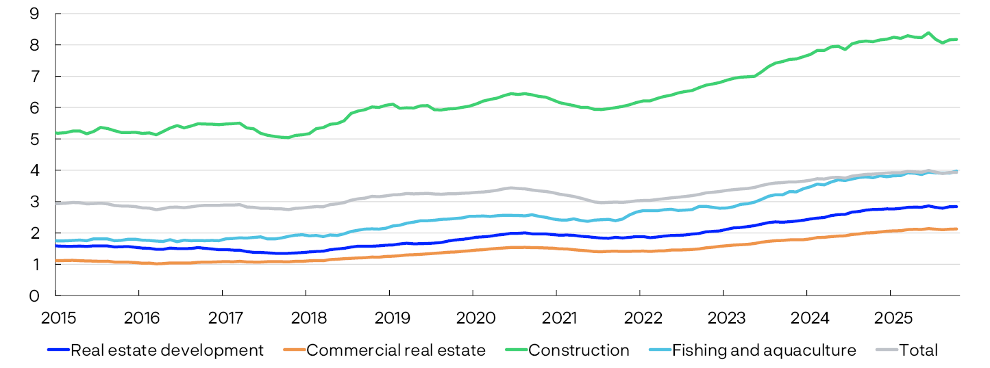
A simple prediction model for developments in the share of bankruptcies one year ahead, based on the share of firms with debt collection cases, indicates a somewhat higher share of bankruptcies than observed so far in 2025 (Chart 3.8). Over the past year, the model has indicated that the share of bankruptcies will remain relatively stable at around 1.5% to 1.6%. The share of bankruptcies is therefore expected to lie between the current level of 1.4% and the prediction interval.
Expected vs. actual bankruptcies within one year. Percent
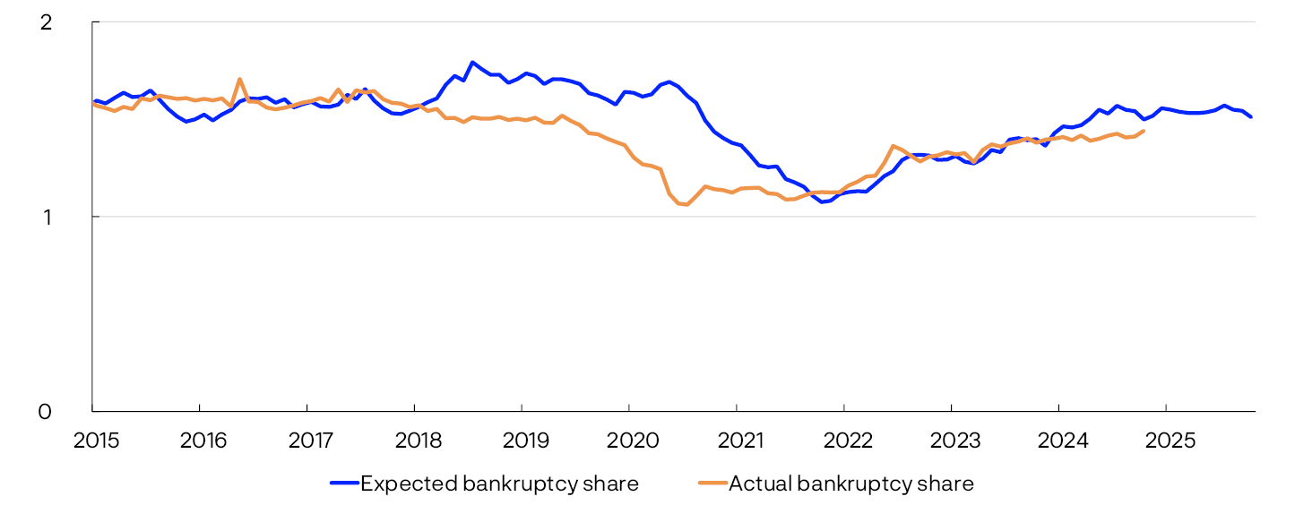
13 Period: January 2015 – October 2025. The share of firms that have gone bankrupt in the past 12 months is the sum of bankruptcies over the past 12 months as a share of the number of firms in the sector over the past 12 months.
14 Period: 2015–2025.
“Two largest bankruptcies” shows the two firms with the highest bank debt in the year of bankruptcy.
For 2025, figures include up to 31 October.
15 See Hjelseth, I. N., and Liaudinskas, K. (2024). “Record Increase in Payment Remarks: A Red Flag for Norwegian Firms?”. Staff Memo 9/2024. Norges Bank.
16 Period: January 2015 – October 2025.
The share of firms with registered debt collection cases is a twelve-month moving average of the number of firms with at least one new debt collection case per month as a share of the number of firms in the sector.
17 Period: January 2015 – October 2025. The share of firms that have gone bankrupt is the sum of bankruptcies over the past 12 months as a share of the number of firms over the past 12 months. The predicted bankruptcy rate is calculated based on the share of firms that go bankrupt within one year after at least one debt collection case (12-month moving average), as well as the share of firms that go bankrupt without having had any debt collection cases in the past year (12-month moving average).
3.4 Low construction activity remains a challenge for real estate developers
High construction costs and higher interest rates have dampened demand for new residential and commercial buildings in recent years. Construction activity has declined, and the earnings of real estate developers and contractors have fallen. Real estate developers are particularly vulnerable because many are highly leveraged and directly affected by higher financing costs. Real estate development loans (planning, organising, execution and the sale of real estate projects) account for about 8% of banks’ Norwegian corporate exposures, which is lower than banks’ CRE exposures, albeit high compared with most other sectors.
Number of new unsold homes is still high and construction activity low
The real estate development market remains challenging, with solvency and liquidity problems reflecting the typical challenges faced by real estate developers in achieving selling prices that cover project costs. Cost growth is primarily driven by higher construction and financing costs (see “Cost components in a typical residential real estate development project”), which have dampened new home sales and resulted in a high number of unsold new homes (Chart 3.9).
Number of unsold new homes
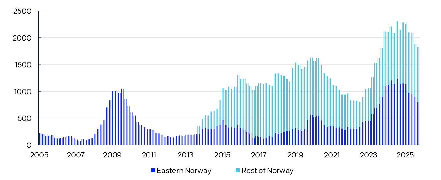
For unsold new homes to be sold without a loss and for new projects to be launched, buyers’ willingness to pay must at least match developers’ costs in addition to a project margin. However, higher interest rates have reduced demand for new homes. At the same time, the price difference between new and existing homes remains somewhat wider than normal, making new homes relatively less attractive. Many projects are therefore not sold. Most developers also depend on external financing from banks, where there is normally a 50% pre-sale requirement. This makes starting construction on new projects difficult.
In the period between 2021 and 2024, interest expenses in real estate development doubled, while earnings halved. This has resulted in a marked decline in the interest coverage ratio (ICR), which measures current earnings as a share of interest expenses. In 2024, the ICR was stable at approximately 1, meaning that total earnings only covered interest expenses exactly (Chart 3.10).
Interest coverage ratio

Developments were somewhat more favourable than expected in Financial Stability Report 2024 H2, but an ICR of 1 is not sustainable. When earnings are insufficient to cover interest expenses, firms must draw on their financial buffers or resort to other measures to avoid defaulting on debt. Risk levels are particularly high for firms that have building plots financed to a large extent by debt and many unsold units.
Somewhat lower financing costs and higher house prices are likely to boost profitability ahead
Prospects indicate that the real estate development market will pick up somewhat. Construction costs are expected to increase less ahead, and lower interest rates are reducing financing costs somewhat. Increased household purchasing power is likely to boost demand for both new and existing homes. The impact on prices is expected to be faster and more significant and faster than in the primary housing market. If the price difference between the two housing markets narrows, new homes will become relatively more attractive.
The stock of unsold new homes remains high but has fallen somewhat since the peak in 2024. Given that the stock of homes is not rising further, this may indicate lower risk for residential property developers and their lenders. In addition, Norges Bank’s Regional Network contacts report some new project launches among financially sound real estate developers. This may be an early sign of market improvement.
However, developments are uncertain. The current situation is eroding liquidity in many firms, and more bankruptcies and higher credit losses are possible ahead. In Norges Bank’s lending survey for 2025 Q3, half of banks report an increased risk of default and breach of the terms of loan covenants in real estate development. See Section 3.6 for a discussion on the outlook for real estate development according to banks.
Cost components in a typical residential real estate development project
When assessing real estate projects, developers weigh various cost components and a margin against expected sales revenue. The calculations for residential and commercial buildings are primarily the same. However, for commercial buildings, the entire building is often sold before or upon completion, frequently with pre-lease contracts. The value is then largely determined by rents and yields. For residential buildings, the revenue side comprises expected income from the sale of the housing units (Chart 3.A).

The cost components in a calculation for a residential real estate development project can be summarised as follows:
- Construction contract cost: Materials and labour. This cost clearly accounts for the largest share of the costs in a development project.
- Land costs: purchase price, stamp duties and registration fees.
- Project owner costs: advisors, project management, sales/marketing, fees/charges and corporate costs.
- Financing costs: interest and costs related to construction loans and land financing.
- Sequencing provisions: costs related to regulatory requirements.
- Project owner costs: advisors, project management, sales/marketing, fees/charges and corporate costs.
In recent years, the construction contract cost has risen considerably, primarily as a result of higher material costs. Material costs have risen by around 55% since 2021, while labour costs have risen by around 18% in the same period. Financing costs have risen in pace with higher interest rates.
Theoretical calculations indicate that land costs have fallen in recent years.1 At the same time, there are few completed transactions that show a clear fall in prices. This may mean that developers are waiting for market conditions to improve, which may dampen construction activity over time.2 Costs related to sequencing provisions and project owner costs have remained relatively stable since 2021, and the margins used by developers in their calculations are likely little changed.3
Longer processing times for zoning plan proposals, in particular in Oslo, affect the property calculation. Increased time from project launch to completion reduces the current value of sales revenues, raises financing costs and may increase costs relating to materials, the project owner and labour. Extended construction time may also trigger new sequencing provisions.
1 Theoretical calculations made by Union in their housing development survey in spring 2025 show that building plot prices for a standard project in Oslo have declined by 12% in nominal terms since the peak in 2021. The calculations are not based on actual transactions, but on house price developments, construction contract costs, project owner costs and financial costs.
2 In Union’s spring 2025 survey, some developers report that they are in a demanding period where they have accepted lower margins in order to launch projects on existing building plots. According to the survey, one possible interpretation is that the value of existing building plots has fallen.
3 See Union’s house development survey from spring 2025 for a more detailed description of cost component and project margin developments.
18 Period: January 2005 – October 2025.
Number of unsold new homes. Not seasonally adjusted. Only pre-2013 figures for Eastern Norway. The data cover all projects with more than 15 housing units. The stock of unsold homes is also affected by some real estate projects being temporarily halted, cancelled, or put back up for sale.
19 Period: 2000–2024.
Actual figures and projections for 2024 for FSR 2024 H2.
In the FSR 2024 H2 projection, the average interest rate was assumed to increase by 1 percentage point in 2024. Furthermore, operating income was assumed to fall by 16% in 2024. Operating costs were assumed to change by 90% of the percentage change in income in both 2024 and 2025. Interest-bearing debt in 2024 was assumed to remain at the same level as in 2023.
Interest coverage ratio (ICR) is earnings (EBITDA) as a share of total interest expenses for legal entities in real estate development.
3.5 Stable outlook for commercial real estate
Banks’ high CRE exposure is a key financial system vulnerability. Higher financing costs and lower property values have exerted pressure on the profitability and solvency of CRE firms. At the same time, most firms have maintained ICRs well above critical thresholds, and default rates have remained low, increasing banks’ willingness to extend CRE loans.
Higher interest rates in recent years have lowered ICRs in the CRE sector (Chart 3.11). In 2024, the ICR fell approximately as projected in Financial Stability Report 2024 H2. Overall, CRE firms’ continued to have ICRs well above 1, ie when earnings are just sufficient to cover interest expenses and these ICRs are also above the minimum requirement of 1.8, which a number of lenders are using.20 Earnings among CRE firms have remained firm owing to a rapid rise in rental income on the back of high employment and inflation adjustments to existing leases. Interest expenses are assumed to have peaked in 2024 and are expected to remain more stable in 2025. Together with a further increase in rental income, this will improve ICRs for CRE firms ahead. In Norges Bank’s lending survey for 2025 Q3, banks report unchanged risk of breach to the terms of loan covenants relating to ICRs and equity ratios.
Interest coverage ratio
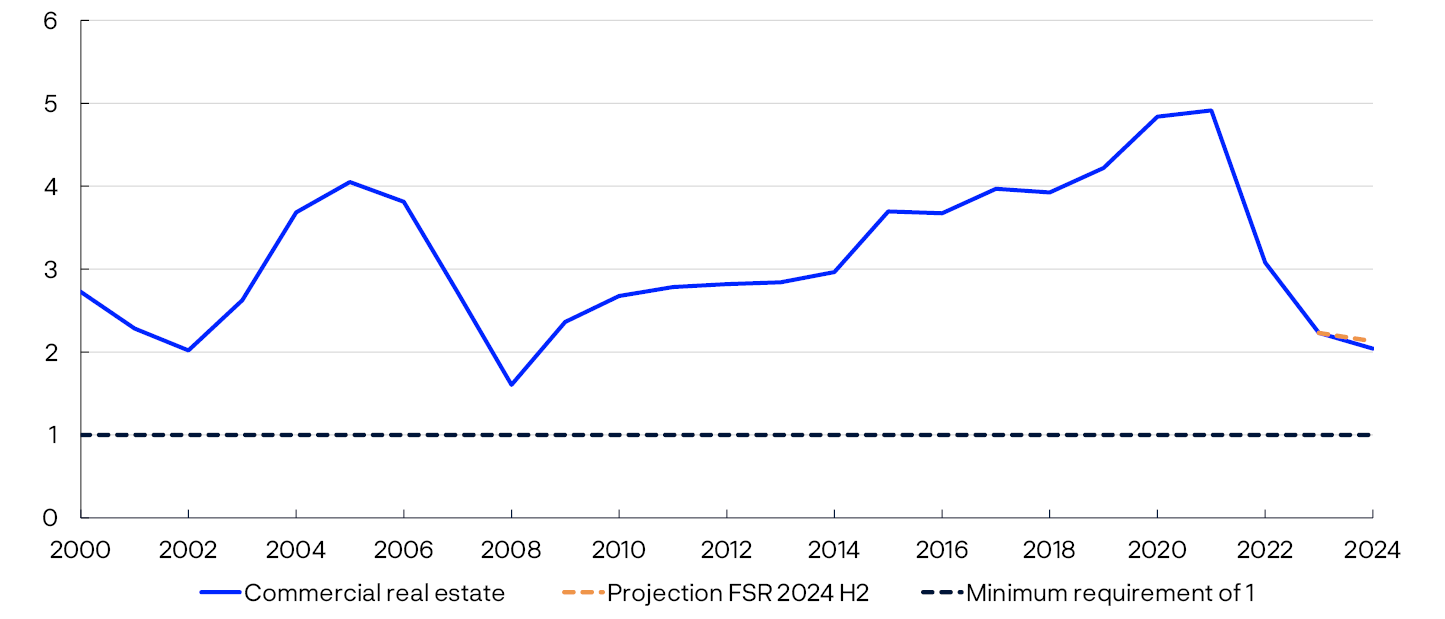
Estimates based on consolidated financial statements22 show that the vast majority of CRE groups were able to cover interest expenses out of current earnings in 2024 (Chart 3.12). CRE groups with ICRs below 1 accounted for just below 12% of debt in 2024, (Chart 3.12). This share is not substantially higher than in 2023, which may be because some groups have reduced debt by selling property.
Share of debt in CRE groups within interest coverage ratio thresholds. Percent

The share of debt held by groups with ICRs below 1 has not increased appreciably, while the share of debt in groups with ICRs between 1 and 3 has increased somewhat (Chart 3.12). This implies that a larger share of debt is held by firms that are more vulnerable. Given that interest expenses have increased somewhat further in 2024, these developments were as expected. At the same time, the shift of debt towards groups with lower ICRs was less pronounced than in the period between 2022 and 2023, suggesting a more moderate rise in credit risk. The CRE sector’s ability to service interest payments is expected to improve ahead and shift debt distribution towards groups with higher ICRs. This indicates more stable CRE prospects.
Since the financial crisis between 2008 and 2009, CRE firms’ overall solvency has strengthened, partly reflecting a rise in commercial property prices without a corresponding rise in lending. Interest rate increases in recent years have led to lower property prices and put pressure on CRE firms’ solvency, resulting in a marked decline in equity ratios in the period between 2022 and 2023 (Chart 3.13). Even if interest expenses increased slightly further in 2024, solvency among CRE firms strengthened somewhat again between 2023 and 2024. The fact that some firms have raised equity or sold off property to pay down debt may have strengthened solvency.
Share of debt in CRE groups within equity ratio thresholds. Percent
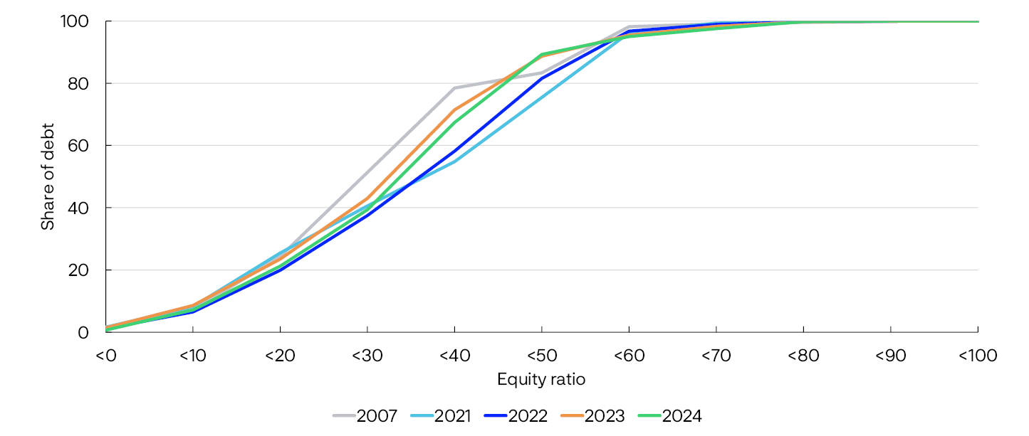
CRE firms have ample access to financing, but equity-financed participants now account for a large share of transactions.
At present, banks’ willingness to lend is strong and there is intense competition between banks to provide CRE loans. In Norges Bank’s lending survey for 2025 Q3, a number of banks reported pressure on spreads and stronger competition, particularly for prime real estate. Credit premiums on CRE firms’ bank and bond financing have fallen from the peak at the end of 2023. For bonds, credit premiums increased slightly at the beginning of 2025 but have continued to fall through 2025. Together with somewhat lower short-term yields, this is dampening financing costs for loans maturing in the coming years.
Even though difficulties in obtaining financing have eased and costs have been reduced, transaction volumes are not particularly high. Market participants report selectivity in the transactions market, where the price expectations of buyers and sellers often differ. Over the past year, the transactions market has been marked by equity-financed participants such as pension funds and insurance companies. These participants have played a role in pushing down the yield to a level that is lower than what leveraged participants can compete with.
Significance of equity investors in the transactions market for commercial real estate
In recent years, equity investors such as pension funds and insurance companies have come to play a more dominant role in the CRE transactions market. In 2025, equity investors have accounted for 70% of transaction volumes for prime office space in Oslo. These investors are motivated by, for example, the need to rebalance portfolios in response to the sharp rise in the equity market. In order to maintain desired asset allocation, this implies, for example, higher real estate investment.
With a long investment horizon and lower dependence on debt financing, equity investors are less vulnerable to interest rate changes. They have also been willing to purchase property when many debt-financed participants have been reluctant to invest, and this has kept transaction volumes and property values buoyant.
At the same time, a strong presence of equity investors entails some potential vulnerabilities. If the equity market were to enter into a steep downturn, these market participants could again abruptly cease to purchase real estate. This could lead to a steep rise in the yield in the market and trigger a fall in commercial property prices. Given that such investors often tend towards longer-term ownership, this could also mean that fewer properties are listed for sale, resulting in a relatively illiquid market.
On the whole, equity investors have nevertheless helped sustain the transactions market and thereby dampened vulnerability in a period of high financing costs.
Selling prices have rebounded somewhat and are expected to remain flat ahead
Commercial property prices fell considerably in 2022 and 2023 owing to higher interest rates. Prices stabilised in 2024 and increased again somewhat in 2025 Q1. Selling prices are estimated as the ratio of market rents to a yield.25 The rise in interest rates resulted in markedly higher yields and a fall in selling prices, while a sharp rise in rents has cushioned the fall in prices. The yield was revised down somewhat in 2025 Q1,26 reflecting that equity-financed participants have had an impact on the market (see “Significance of equity investors in the transactions market for commercial real estate”).
The interest rate outlook suggests that yields are likely to remain fairly flat. Moreover, equity investors are expected to continue to purchase more properties, albeit to a somewhat lesser extent than before. This will result in slightly weaker competition, and more transactions are expected to be carried out by leveraged participants at somewhat lower prices, which leads to a slightly higher yield ahead. Should the equity investors divest from the market to a greater extent than assumed, this would suggest a somewhat higher yield than currently projected.
The rise in nominal rents has been sharp for a long period, driven by high employment and low office vacancy rates. So far in 2025, however, developments in nominal rents have been stable and somewhat lower than projected in the May Report. Even though employment is high, office vacancy rates have recently edged up slightly. Market participants report that demand for office space has weakened somewhat owing to heightened uncertainty. In addition, more large projects will be completed that are also likely to push up office vacancy rates somewhat ahead. Overall, rents are therefore expected to rise more moderately than in recent years.
On the whole, the projections for rent inflation and the yield imply that commercial property selling prices will remain fairly flat (Chart 3.14). These prices are expected to remain at a slightly higher level in the coming years than expected in the May Report, but they will be fairly similar at the end of the projection period.
Prime real estate in Oslo. Estimated selling prices. In thousands of NOK per square meter
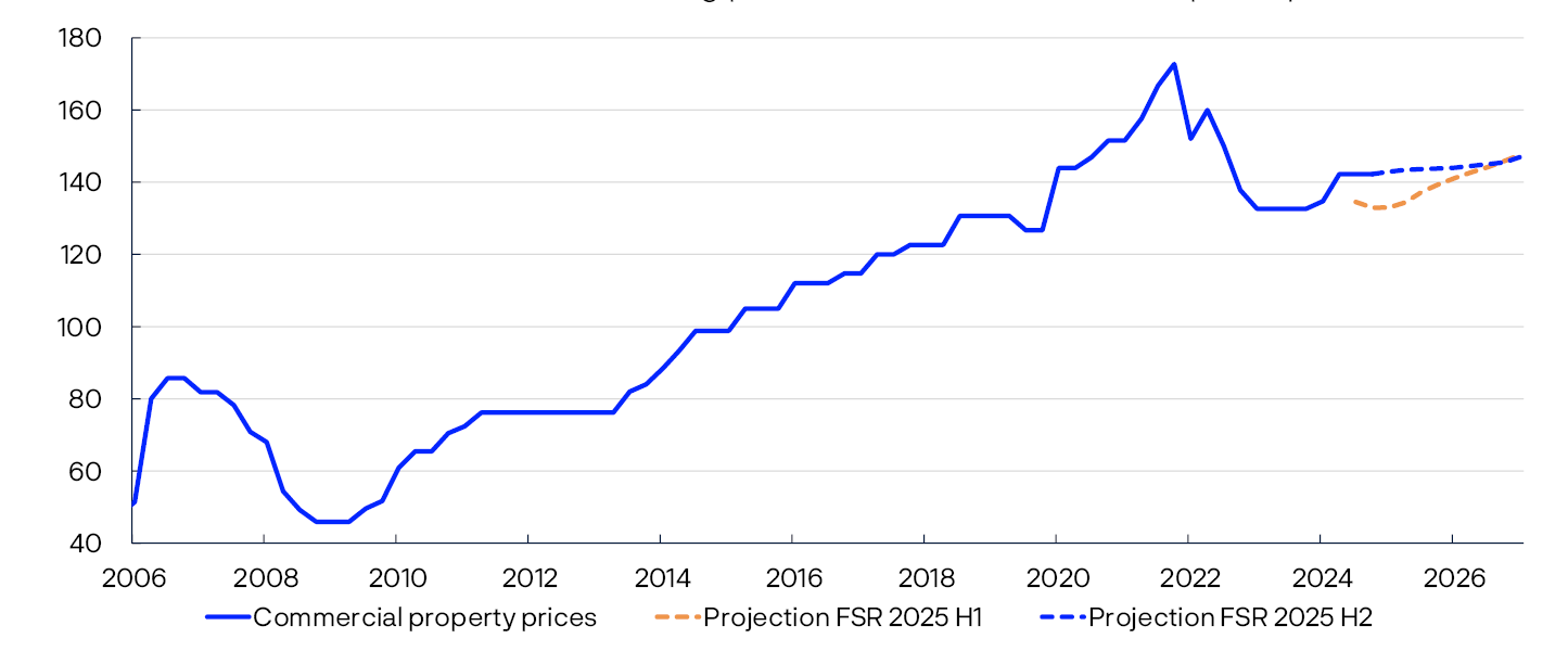
20 For firms that rely on bond financing, some credit rating agencies require an ICR above 1.8 to qualify for a high credit rating. If the ICR falls below this threshold, the bonds may be downgraded, with a marked rise in yields on new and existing bonds.
21 Period: 2000–2024. Projection from 2024 for FSR 2024 H2.
Interest coverage ratio is total earnings as a share of total interest expenses for legal entities in commercial real estate.
In the FSR 2024 H2 projection, the average interest rate was assumed to increase by 0.6 percentage point in 2024. Furthermore, operating income was assumed to increase by 4.7% and operating costs was assumed to increase by 3.2% in 2024. It was also assumed that interest-bearing debt would increase by 3.5 % in 2024.
22 Consolidated financial statements provide a more comprehensive picture of the financial situation than financial statements at firm level and are therefore better suited for micro-level analyses.
23 Period: 2022–2024. Interest coverage ratio is total earnings as a share of total interest expenses. The sample comprises CRE groups with interest-bearing debt over NOK 50m.
24 Period: 2007, 2021, 2022, 2023, 2024. Equity ratio is total book equity as a share of total book assets (equity and debt) for CRE groups.
25 This yield is not the same as investors’ actual required rate of return but is the yield set by market participants on the basis of information from real estate sales and market rents for those same properties. In general, investors’ required rate of return and therefore selling prices depend on developments in long-term interest rates and risk premiums.
26 The yield reduction is a revision of the historical data. According to Financial Stability Report 2025 H1, the yield was 4.75% in 2025 Q1, which explains why selling prices are now considerably higher in the beginning of the projection period compared with the May Report.
27 Period: 2006 Q4 – 2027 Q4. Projections from 2025 Q2 for FSR 2025 H1 and from 2025 Q4 for FSR 2025 H2.
Prime real estate in Oslo is high-quality office buildings located in Vika and Aker Brygge. Selling prices are calculated as rental prices divided by the estimated yield. The yield is based on information from real estate transactions and depends on developments in long-term interest rates and risk premiums.
3.6 Slightly higher losses on corporate exposures expected ahead
In 2025 H1, banks’ total losses on Norwegian corporate exposures remained low and in line with 2024 levels (Chart 3.15).
Recognised credit losses as a share of lending to the sector. Percent
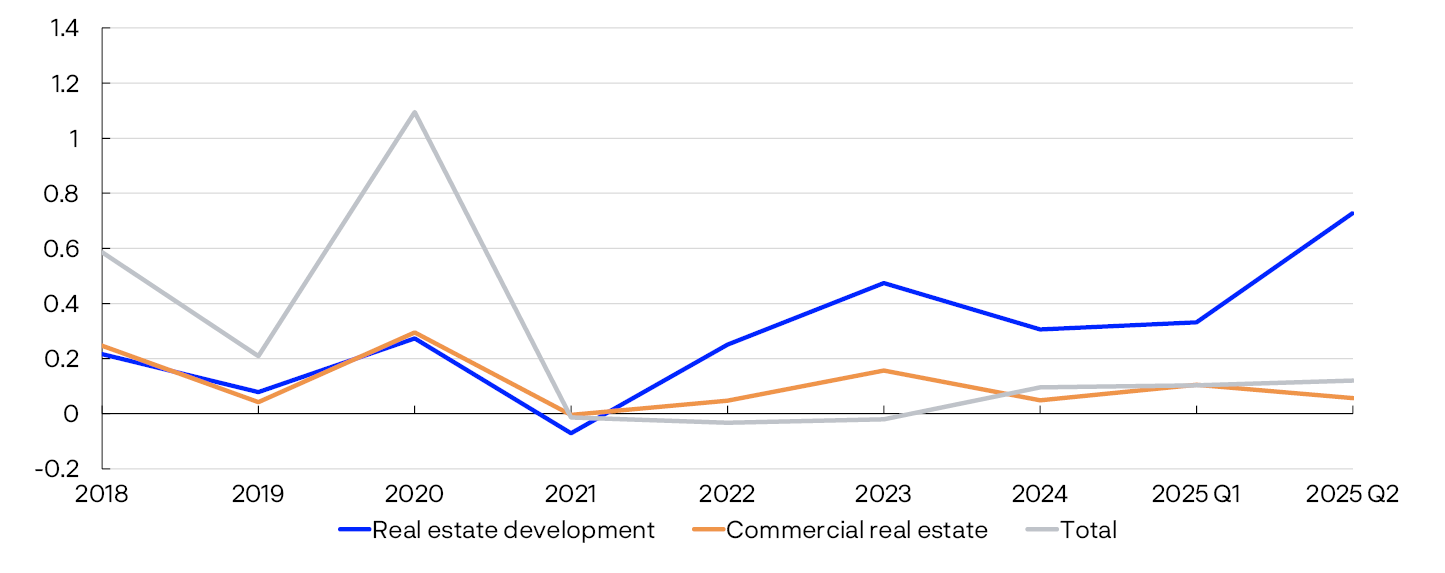
In 2024, losses on CRE exposures fell and were lower than expected. In the first half of 2025, however, credit losses in real estate development rose markedly again. Even though losses in 2024 were lower than expected, the share of defaulted loans in the sector rose further, (Chart 3.16). The default rate is well above the average for the past decade.
Loan defaults as a share of lending to the sector. Percent
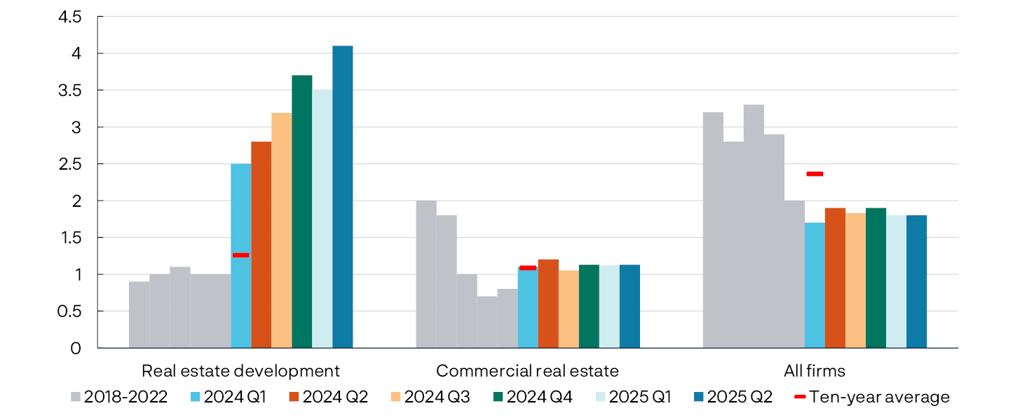
As expected, losses on CRE exposures have remained low, and the share of defaulted loans has remained low and stable. For exposures elsewhere, such as in oil-related and transport sectors, default rates have fallen substantially since 2021. This results in a total share of defaulted loans that is considerably lower than four years ago.
Overall losses on corporate exposures are expected to increase slightly in 2025 and 2026 compared with 2024 (Chart 3.17). Continued low construction activity is expected to result in higher losses on real estate development exposures.30 Improved economic developments lead to a marginal downward adjustment of loss projections compared with the projections in Financial Stability Report 2024 H2.
Loss provisions on new loan defaults as a share of total lending to the sector. Percent
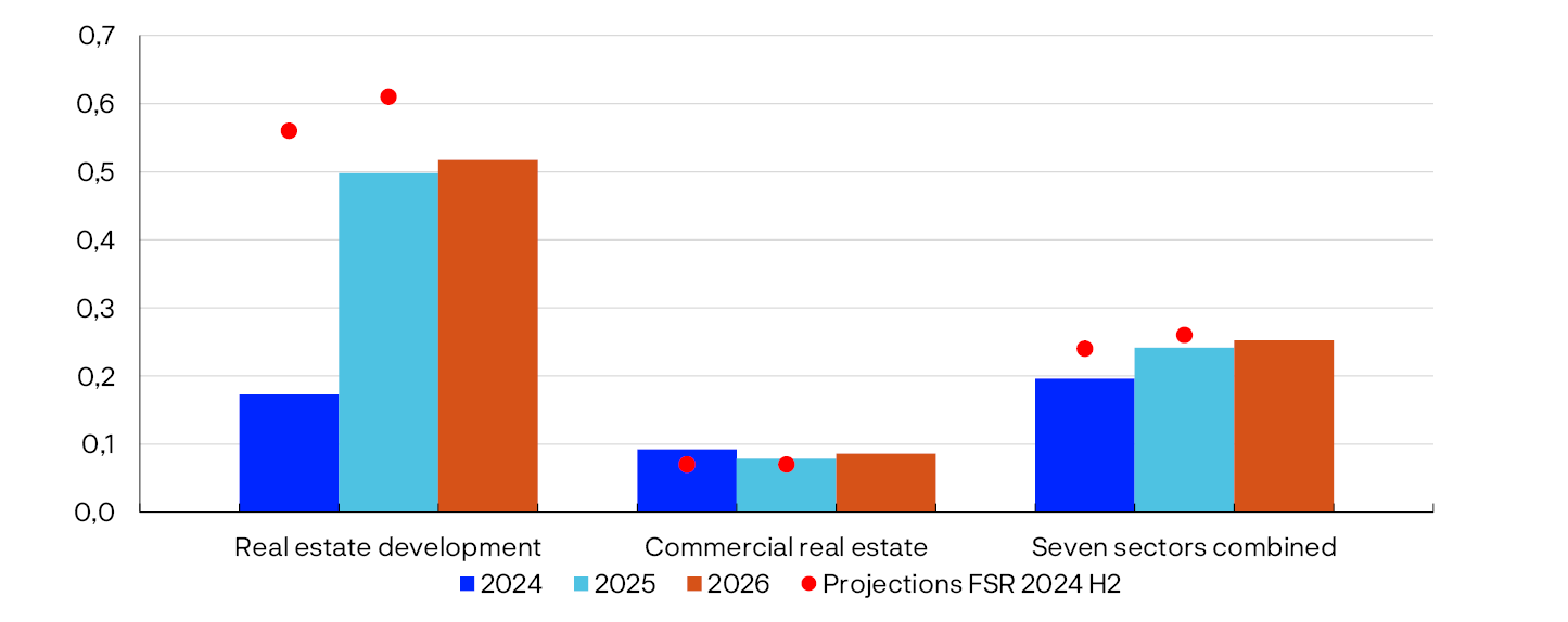
Owing to prospects for somewhat lower financing costs and higher earnings, CRE losses are expected to remain low, at around current levels. The projections have not changed substantially since 2024.
The projections are uncertain and losses may become higher than expected. If unsold new homes remain unsold and construction activity fails to pick up as expected, then more real estate developers could default on their loans and banks could face higher losses on their real estate development exposures than assumed.
The global growth outlook is considerably uncertain. Should long-term interest rates and risk premiums increase markedly, both debt servicing capacity and CRE property values could weaken. Should employment also fall markedly and rental income prove appreciably lower than envisaged, many CRE firms could face difficulties servicing debt and refinancing loans. In a situation where the profitability of many firms has been weakened by higher financing costs, this could trigger more property fire sales. This could lead to higher default rates and losses than envisaged.
28 Period: 2018 – 2025 Q2.
Annual figures for 2018–2024. Annualised figures for 2025 Q1 and Q2. Norwegian exposures only.
29 Period: Figures for 2018 Q4 – 2023 and quarterly figures from 2024 Q1 – 2025 Q2.
”Loan defaults” are the holdings of non-performing loans after 90 days and other defaults as a share of total lending to the sector. Norwegian exposures only.
30 The projections are based on a model that estimates default probabilities at firm level (see Hjelseth et al. (2024). “New microdata on corporate loan defaults improve the estimates of banks’ credit losses” Staff Memo 10/2024. . Norges Bank aims to model loan loss provisions on new corporate loan defaults (new loans in stage 3 according to IFRS 9). Even if there is a central driver of banks’ credit loss recognitions, the actual recognised losses are more complex. For example, while changes in loss provisions in stages 1 and 2 also affect recognised losses, this is not included in Norges Bank’s modelling system. Nevertheless the model estimates are well in line with the Bank’s assessment of banks’ risk of losses and are consistent with the projections from the Bank’s VAR model for total credit losses.
31 Period: 2024–2026. The figure for 2024 is a calculated variable for new loss provisions based on actual new loan defaults for nine large banks and the provision rate on loan defaults at the end of 2024. Projections for 2025 and 2026. The seven sectors are fisheries and aquaculture, manufacturing, construction, retail trade, commercial real estate, real estate development and services. The remaining sectors (oil-related industries, foreign shipping, power, agriculture and forestry) are not included in the data. The projections cover about 80% of banks’ lending to Norwegian firms.